Data Structures for Muggles

CX3302024-08-292024-11-21

Prologue

All the following example will be shown in C Programming Language or pseudo code.

This is the note when I was taking the course in NCKU, 2024. Blablabla…

Finally, I would like to declare that almost every photo I use comes from the handouts of my course at NCKU, provided by the professor. If any photo comes from another source, I will give proper credit in the caption or description of the image.

Complexity

Space Complexity

The amount of memory that it needs to run to completion.
$S(P)=c+S_P(I)$
Total space requirement = Fixed space requirement + Variable space requirements
We usually care more about the Variable space requirements.

For example, we have the following code like this.

Iterative

float sum(float list[], int n)
{
    float tempsum=0;
    int i;
    for (i = 0; i < n; i++){
        tempsum += list[i];
    }
    return tempsum;
}

In this code, we DO NOT copy the array list, we just passes all parameters by value, so the variable space requirements $S_{sum}(I)=0$ . Here’s another example, let’s look at the code first.

Recursive

float rsum(float list[], int n)
{
    if (n) return rsum(list,n-1)+list[n-1];
    return 0;
}

In this case, 1 recursive call requires K bytes for 2 parameters and the return address. If the initial length of list[] is N, the variable space requirements $S_{rsum}(N)=N\times K$ bytes.

Time Complexity

The amount of computer time that it needs to run to completion.
$T(P)=c+T_P(I)$
Total time requirement = Compile time + Execution time
We usually care more about the Execution time.

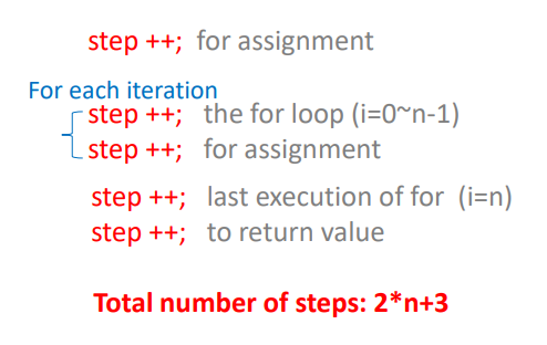
For example, this is a segment with execution time independent from the instance characteristics.

float sum(float list[], int n)
{
    float tempsum=0;
    int i;
    for (i = 0; i < n; i++){
		tempsum += list[i];
    }
    return tempsum;
}

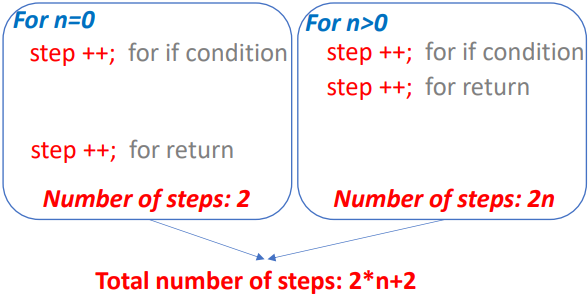
On the other hand, a segment with execution time dependent on the instance characteristics will be like this.

float rsum(float list[], int n)
{
    if (n){
         return rsum(list,n-1)+list[n-1];
    }
    return 0;
}

For given parameters, computing time might not be the same. So, we should know the following cases.

Best-case count: Minimum number of steps that can be executed.
Worst-case count: Maximum number of steps that can be executed.
Average count: Average number of steps executed.

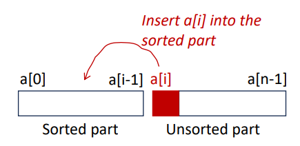
Here, I’m going to use insertion sort to show you the difference between the best-case & the worst-case. If you don’t know what it is, you can go check it out here. Following is a snippet of the insertion sort algorithm in C.

for (j = i - 1; j >= 0 && t < a[j]; j--){
	a[j + 1] = a[j];
}

Worst-case

a[0 : i-1] = [1, 2, 3, 4] and t = 0
- 4 compares
a[0 : i-1] = [1, 2, 3, …, i] and t = 0
- i compares

For a list in decreasing order, the total compares will be

$1+2+3+4+\dots+(n-1)=\frac{n(n-1)}{2}=\frac{1}{2}n^2-\frac{1}{2}n$

Best-case

a[0 : i-1] = [1, 2, 3, 4] and t = 5
- 1 compare
a[0 : i-1] = [1, 2, 3, …, i] and t = i + 1
- 1 compare

For a list in increasing order, the total compares will be

$1+1+1+\dots+1=n-1$

Asymptotic Complexity

Sometimes determining exact step counts is difficult and not useful, so we will use the Big-O notation to represent space and time complexity. Here’s a question, which algorithm is better? The one with $\frac{1}{2}n^2-\frac{1}{2}n$ or $n^2+3n-4$ . The answer is, both of them are $O(n^2)$ , so the performances are similar.

Now, we jump back to the example in previous part. What is the time complexity of insertion sort in the Big-O representation?

Worst case
- $\frac{1}{2}n^2-\frac{1}{2}n\Rightarrow O(n^2)$
Best case
- $n-1\Rightarrow O(n)$

Why Algorithm Is Important

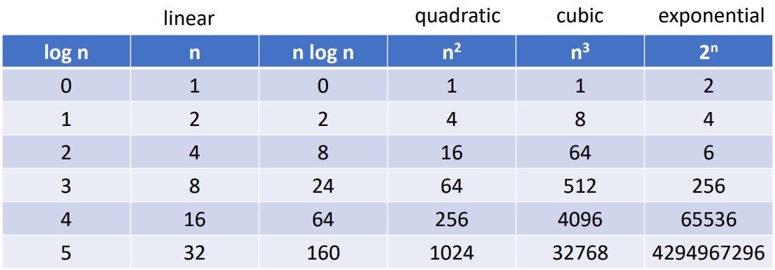
This is a table of how various functions grow with $n$ .

As you can see, the exponential one grows exponentially, which means a little variation of n can increase a lot of computing time. In fact, on a computer performing 1 billion (109 ) steps per second. $2^{40}$ steps require 18.3 mins, $2^{50}$ steps require 13 days, and $2^{60}$ steps require 310 years! So that’s why improving algorithm may be more useful than improving hardware sometimes.

Summary

Space and time complexity
- Best case, worst case, and average
- Variable and fixed requirements
Asymptotic complexity
- Big-O
Example:
- Insertion sort
- Selection sort

More information about complexity will be introduce when I take the algorithm course next year, or you can search for some sources if you really want to learn more about it.

Arrays

Intro

It’s a collection of elements, stored at contiguous memory locations. Each element can be accessed by an index, which is the position of the element within the array. It’s the most fundamental structure and the base of other structures.

1-D Array

This is an 1-D array with length 10. We can access the first element by the index 0 (zero-indexing). But what should we do if the memory size we need is changing and not always the same? Will it be suitable for all kind of situation?

The answer is negative, and that’s why we need something called Dynamic Memory Allocation. When we need an area of memory and do not know the size, we can call a function malloc() and request the amount we need. The following is an code implementation of a dynamic 1-D array storing integers.

int size;
scanf("%d", &size); // Ask an arbitrary positive number as the size of the array
int *array = (int *)malloc(size * sizeof(int)); // Finish the memory allocation

// Do operations to the array here

free(array); // Free the memory after use

The free() function deallocates an area of memory allocated by malloc().

So, that’s how to implement the dynamic 1-D array in C. Now, here comes another question. What if we want to store some data like the student ID and his exam scores? Should we store it in an 1-D array?

2-D Array

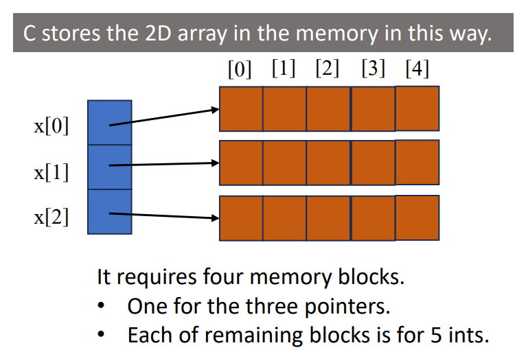
To answer the question above, we can choose 2-D array as the data structure to store something like that. C uses array-of-array representation to represent multidimensional array. The following is an example diagram to show how the things work in an 2-D array in C.

To be more specific, it shows that the first dimension of the array (blue part) stores the pointers that pointing to the second dimension arrays (orange part), which are storing integer or other data types. Following is an example code of a dynamic 2-D array.

int rows, cols;

// Get the dynamic size
scanf("%d", &cols);
scanf("%d", &rows);

// Allocate the first dimension (blue part in the diagram above)
int **array = (int **)malloc(cols * sizeof(int *));
// For every rows, allocate the rows size for the row (orange part)
for (int i = 0; i < cols; i++) {
    array[i] = (int *)malloc(rows * sizeof(int));
}

Row-Major and Column-Major

To know what is row-major & column-major, we can take a look at this example. If we have a matrix called A.

$A=\left[\begin{array}{lll}1 & 2 & 3 \\ 4 & 5 & 6 \\ 7 & 8 & 9\end{array}\right]$

Column-major
- $A=[1, 4, 7, 2, 5, 8, 3, 6, 9]$
- Elements of the columns are contiguous in memory
- Top to bottom, left to right
- Matlab
- Fortran
Row-major
- $A=[1, 2, 3, 4, 5, 6, 7, 8, 9]$
- Elements of the rows are contiguous in memory
- Left to right, top to bottom
- C
- C++

Stacks

Intro

Stack is also an fundamental structure that is opposite from Queue (will be mentioned later), it has some properties

Last-In-First-Out (LIFO)
Like a tennis ball box
Basic operations
- Push: Insert an element to the top of the stack
- Pop: Remove and return the top element in the stack
- Peek/Top: Return the top element in the stack
- IsEmpty: Return true if the stack is empty
- IsFull: Return true if the stack is full

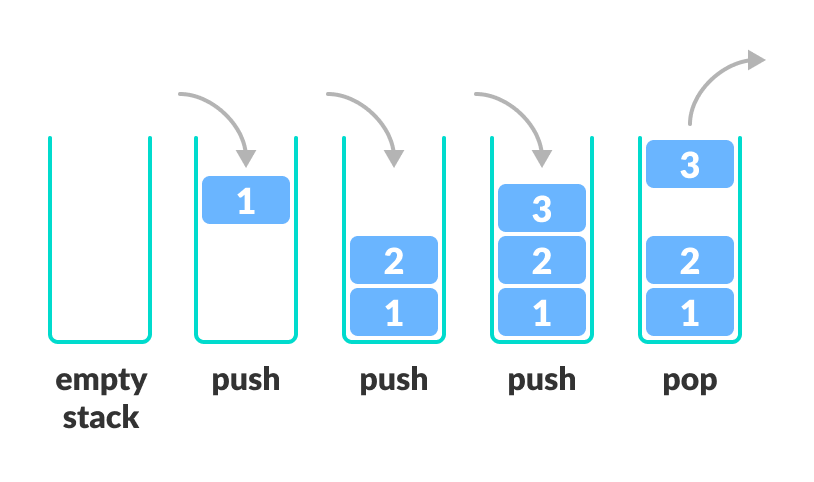
The following is the diagram of the push and pop operation of stacks.

Application: Balanced Brackets

Check whether the brackets are balanced.
Examples:
- “]” → False
- “(a+b)*c-d” → True
Steps:
- Scan the expression from left to right
- When a left bracket, “[”, “{”, or “(”, is encountered, push it into stack.
- When a right bracket, “]”, “}”, or “)”, is encountered, pop the top element from stack and check whether they are matched.
  - If the right bracket and the pop out element are not matched, return False.
- After scanning the whole expression, if the stack is not empty, return False.

Dynamic Stacks

If we want to dynamically allocate the size of the stack, we should still use malloc(). Here’s an example using dynamic arrays.

Headers and declarations

int *stack;
int capacity = 1; // Initial capacity
int top = -1; // Representing empty stack

Create stack

void createStack() {
    stack = (int*)malloc(capacity * sizeof(int));
    if (stack == NULL) {
        printf("Memory allocation failed\n");
        exit(1);
    }
}

Array doubling when stack is full

void stackFull() {
    capacity *= 2;  // Double the capacity
    stack = (int*)realloc(stack, capacity * sizeof(int));
    if (stack == NULL) {
        printf("Memory allocation failed\n");
        exit(1);
    }
    printf("Stack expanded to capacity: %d\n", capacity);
}

Check if the stack is empty

int isEmpty() {
    return top == -1;
}

Push

void push(int value) {
    if (top == capacity - 1) {  // If the stack is full, double it
        stackFull();
    }
    stack[++top] = value;
}

int pop() {
    if (isEmpty()) {
        printf("Stack underflow. No elements to pop.\n");
        return -1;
    }
    return stack[top--];
}

Peek (or Top)

int peek() {
    if (isEmpty()) {
        printf("Stack is empty.\n");
        return -1;
    }
    return stack[top];
}

Queues

Intro

As I mentioned, queues are the opposite of stacks. That is because although they are both linear or ordered list, they have totally different properties.

First-In-First-Out (FIFO)
New elements are added at the rear end
Old elements are deleted at the front end.
Basic operations
- Enqueue
  - Insert element at the rear of a queue
- Dequeue
  - Remove element at the front of a queue
- IsFull
  - Return true if the queue is full. (rear == MAX_QUEUE_SIZE - 1)
- IsEmpty
  - Return true if the queue is empty (front == rear)

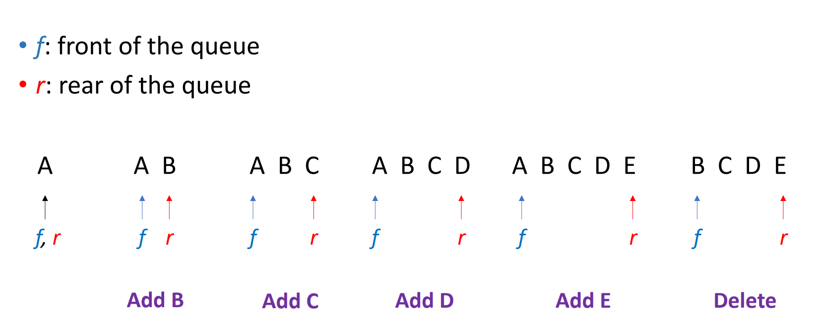
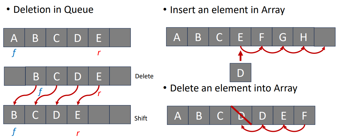
The following is the diagram of the insertion and deletion of the queues.

If now e have a queue that contains 5 elements but has the length 6 (null stands for no element there).

$Q = [A, B, C, D, E, null]$

After we delete an element from the front and add another one at the rear, it will be like this.

$Q = [null, B, C, D, E, F]$

The queue will be regarded as full since rear == MAX_QUEUE_SIZE, but we know that actually some empty space remains. So, how to fix it? We can think about when a customer at front of the line leaves, what will other customers do?

They move forward. So, we should shift other elements forward after deletion. That way, the queue became

$Q = [B, C, D, E, F, null]$

Voila! We fix it! But if we do this at every deletion, the program will be way too slow. So here’s the next question, what should we do to fix it?

Circular Queue

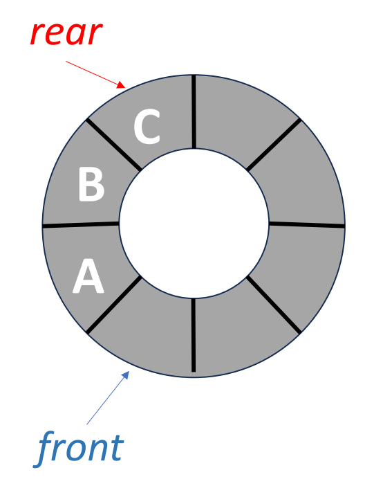
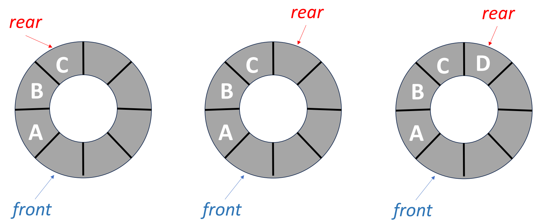
In a circular queue, the front and the rear will have some differences comparing with the normal queue.

front: One position counterclockwise from the position of the front element.
rear: The position of the rear element.

This is how it looks like.

The addition or insertion in an circular queue has the following steps:

Move rear one position clockwise:
rear = (rear + 1) % MAX_QUEUE_SIZE
Put element into queue[rear]

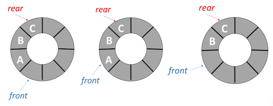
And the deletion steps are below:

Move front one position clockwise:
front = (front + 1) % MAX_QUEUE_SIZE
Return and delete the value of queue[front]

In a circular queue, how to know a queue is full? We can think about when a queue is keep adding elements until it’s full, what will the front and rear go? The answer is, when elements are keep being added to a circular queue, the rear will keep going clockwise and finally equals to the front.

On the other hand, we can also use this to determine if the queue is empty. Because if the elements in the queue are keep being deleted, the front will keep moving clockwise until it equals to rear.

So if the condition to determine the full and empty are the same (front == rear), how can we tell which is which?

Here’s some of the solutions, but there are still a lot of ways to conquer this.

Set a LastMoveIsFront() boolean value to recognize the last move is front or rear.
Set another variable count and modify it everytime we delete or add something.
Save an empty slot in the circular queue, so that when the queue is full, the rear will be at the position “just before the front” (because one empty slot is reserved), thus avoiding the confusion with the condition rear == front which indicates an empty queue.

Linked Lists

Intro

First, I want to talk about the deletion and insertion in sequential representation, which is mentioned a lot in the previous parts. When we deleting or inserting things in a queue or an array, there’re always be some empty spaces created by the operations (See the picture below for details.) And that means we have to move many elements many times to maintain a sequential data structure.

So, to avoid this waste, we want to store data dispersedly in memory, just like the picture below.

But now, we are facing another problem. How do we know the order of the data if we store an sequential data like this? We use linked list! Let’s start talking about linked list right away. Here is the features of it.

In memory, list elements are stored in an arbitrary order.
The fundamental unit is called a node.
In a normal linked list, a node contains data and link/pointer.
The link is used to point to the next element.

To answer the previous question, we need to talk about why linked list is called linked list. It’s because every element in the list linked to the very next data, so we can know the sequence even thought we didn’t save them sequentially. To let you better understand, the following graph is the illustration of how it works.

Another way that usually seen to draw a linked list is like this.

Operations

Concept of Insertion

To insert K between B and C, we have to follow the steps below.

Get an unused node a.
Set the data field of a to K.
Set the link of a to point to C.
Set the link of B to point to a.

Concept of Deletion

To delete C in the linked list, we have to follow the steps below.

Find the element precedes C.
Set the link of the element to the position of D.

Define A Node in C

typedef struct listNode *listPointer;
typedef struct {
    char data;
    listPointer link;
} listNode;

Get(0)

desiredNode = first; // get the first node
return desiredNode->data;

Get(1)

desiredNode = first->link; // get the second node
return desiredNode->data;

Delete “C”

Step 1: find the node before the node to be removed

beforeNode = first->link;

Step 2: save pointer to node that will be deleted

deleteNode = beforeNode->link;

Step 3: change pointer in beforeNode

beforeNode->link = beforeNode->link->link;
free(deleteNode);

Insert “K” before “A"

Step 1: get an unused node, set its data and link fields

MALLOC( newNode, sizeof(*newNode));
newNode->data = ‘K’;
newNode->link = first;

Step2: update first

first = newNode

Insert “K” after “B”

beforeNode = first->link;
MALLOC( newNode, sizeof(*newNode));
newNode->data = ‘K’;
newNode->link = beforeNode->link;
beforeNode->link = newNode;

Circular Linked List

The last node points to the first node.

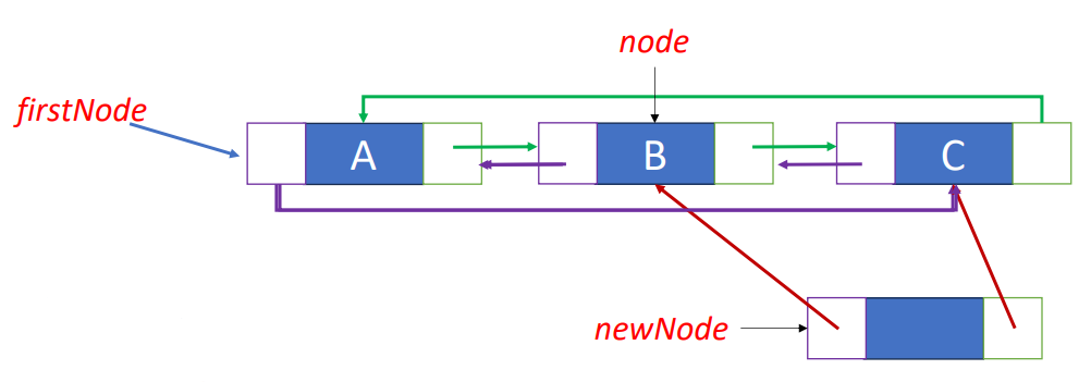
Doubly Linked List

In general linked list, to find an element will always start at the beginning of the list, but it’s not the case in doubly linked list!

Right link: forward direction
Left link: backward direction

Node in Doubly Linked List

typedef struct node *nodePointer;
typedef struct node{
    nodePointer llink;
    element data;
    nodePointer rlink;
};

Insert “K” after “B”

newNode->llink = node;
newNode->rlink = node->rlink;

node->rlink->llink = newNode;
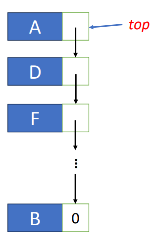
node->rlink = newNode;

Linked Stacks & Queues

Linked stack
- Push: add to a linked list
- Pop: delete from a linked list
Linked queue
- AddQ: add to a rear of a linked list
- DeleteQ: delete the front of a linked list

Summary

Linked lists
Doubly linked lists
Doubly circular linked lists
Operations: Get, Insert, and Delete
Applications:
- Linked stacks
- Linked queues

Trees & Binary Trees

Intro

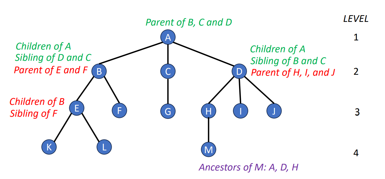
Tree is an data structure that looks like a genealogy, so there’s a lot of terms that similar to the terms in a family. Now, let’s introduce some terms about the trees.

Degree of a node
- number of subtrees
Degree of a tree
- maximum of the degree of the nodes in the tree
Height (depth) of a tree
- maximum level of any node in the tree
Leaf (or Terminal)
- nodes having degree zeros
Internal node
- not leaf & not root
Children
- roots of subtrees of a node X
Parent
- X is a parent
Sibling
- children of the same parent
Ancestor
- all the nodes along the path from the root to the node

List Representation

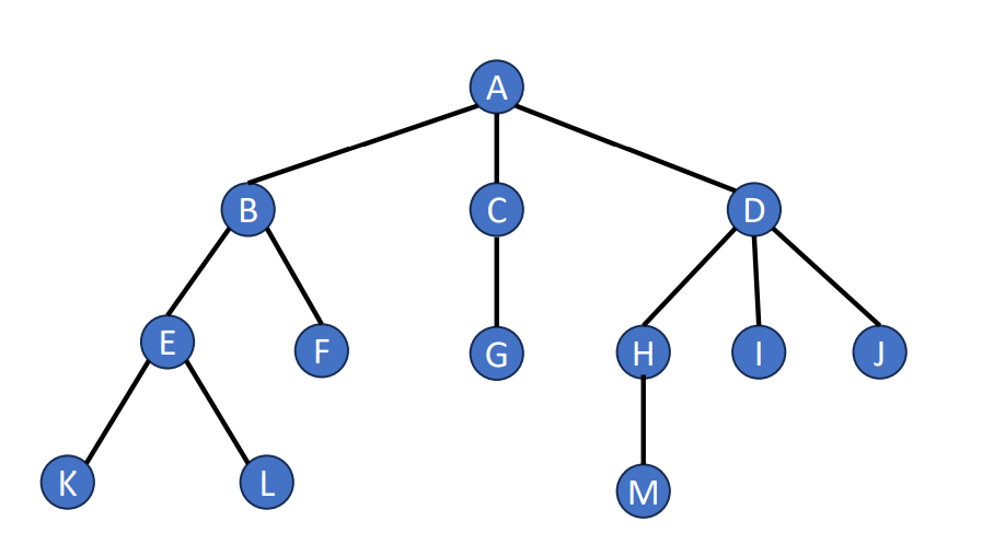
If we want to represent a tree in a list format, we can use this mathod. Following is an example of a tree and its list representation.

It’s list representation will be like $\text{(A (B (E (K, L), F), C (G), D (H (M), I, J)))}$ .

Binary Trees

Binary trees are trees that have the following characteristics.

Degree-2 tree
Recursive definition
- Each node has left subtree and/or right subtree.
- Left subtree (or right subtree) is a binary tree.

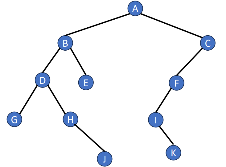
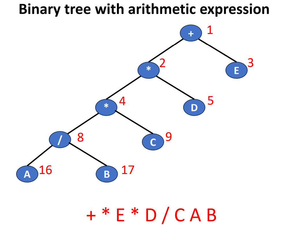
This is an picture of a binary tree.

Full Binary Trees & Perfect Binary Trees

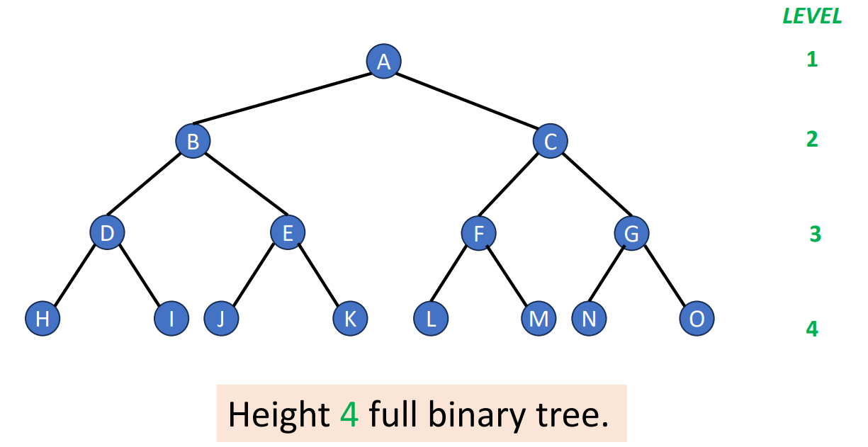
Full Binary Tree
- A full binary tree is a binary tree with either $0$ or $2$ child nodes for each node
Perfect Binary Tree
- A full binary tree
- A tree that has height $h$ and $2^h-1$ nodes

Please note that each perfect binary tree of the same height will only have one type. If we numbering the nodes in a perfect binary tree from top to bottom, left to right, then we will have the following properties.

Let $n$ $n$ be the number of nodes in a perfect binary tree
- Parent node of $i$ is node $floor(\frac{i}{2})$
- Left child of node $i$ is node $2i$
- Right child of node $i$ is node $2i+1$

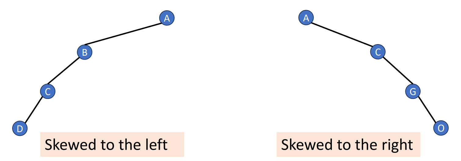
Skewed Binary Trees

At least one node at each of first $h$ levels
Minimum number of nodes for a height $h$

Number of Nodes and Height

Let $n$ $n$ be the number of nodes in a binary tree whose height is $h$ $h$ .
- $h\le n\le 2^h-1$
- $\log_2(n+1)\le h$
- The height $h$ of a binary tree is at least $log_2(n+1)$

Complete Binary Trees

How to create a complete binary tree? Just follow the steps and check out the graph below.

Create a full binary tree which has at least $n$ nodes
Number the nodes sequentially
The binary tree defined by the node numbered $1$ through $n$ is the n-node complete binary tree

Binary Tree Representations

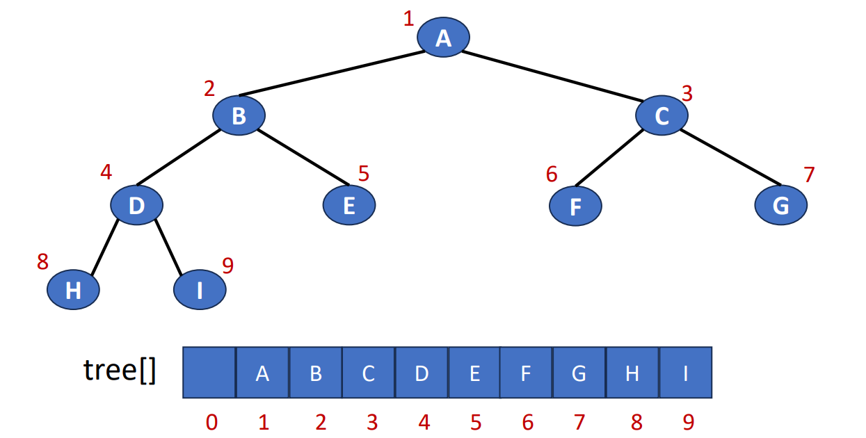
Array Representation

Number the nodes using the numbering scheme for a full binary tree. The node that is numbered i is stored in tree[i].

Since the number should be placed in the FULL binary tree, sometimes there will be some memory waste. For example, if we create a 4-level right-skewed binary tree, it will has the length 15, but only 4 being used.

In array representation, the tree will has the following properties.

Let $n$ be the number of nodes in a tree
- Parent node of $i$ is node $floor(\frac{i}{2})$
- Left child of node $i$ is node $2i$
- Right child of node $i$ is node $2i+1$

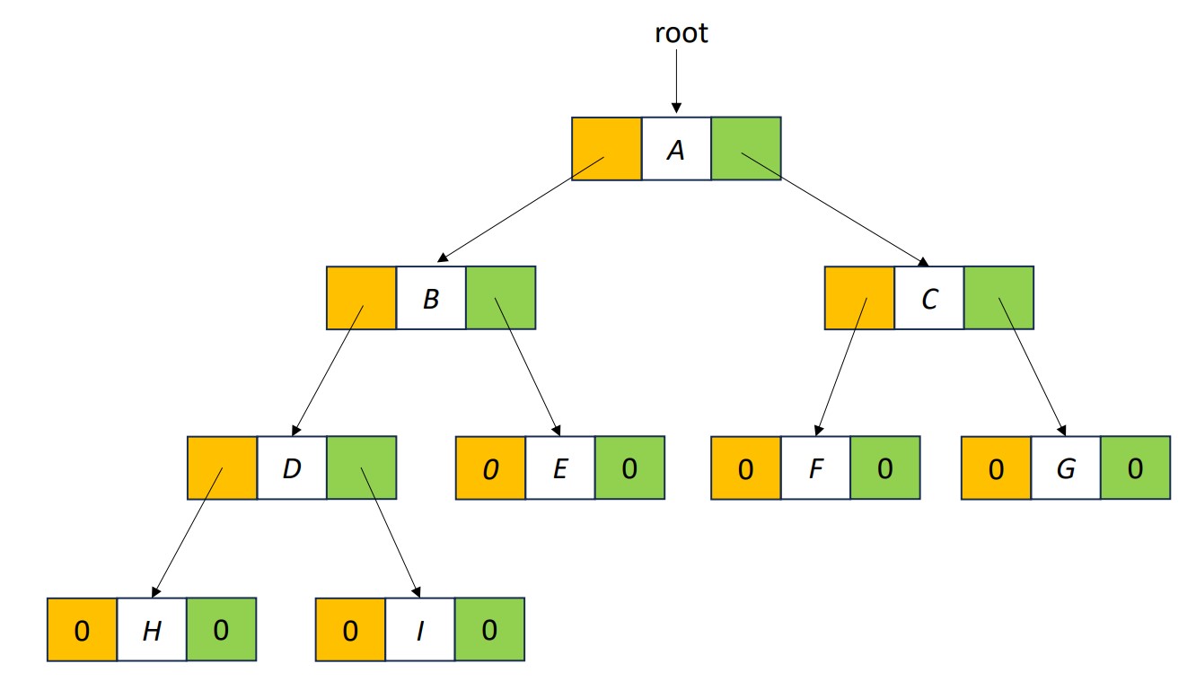
Linked Representation

Each binary tree node is represented as an object whose data type is TreeNode.
The space required by an n node binary tree is n * (space required by one node).

typedef struct node *treePointer;
typedef struct node{
    char data;
    treePointer leftChild, rightChild;
};

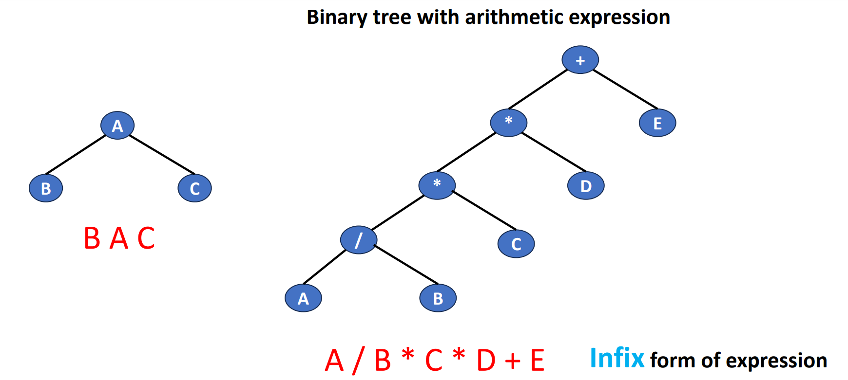
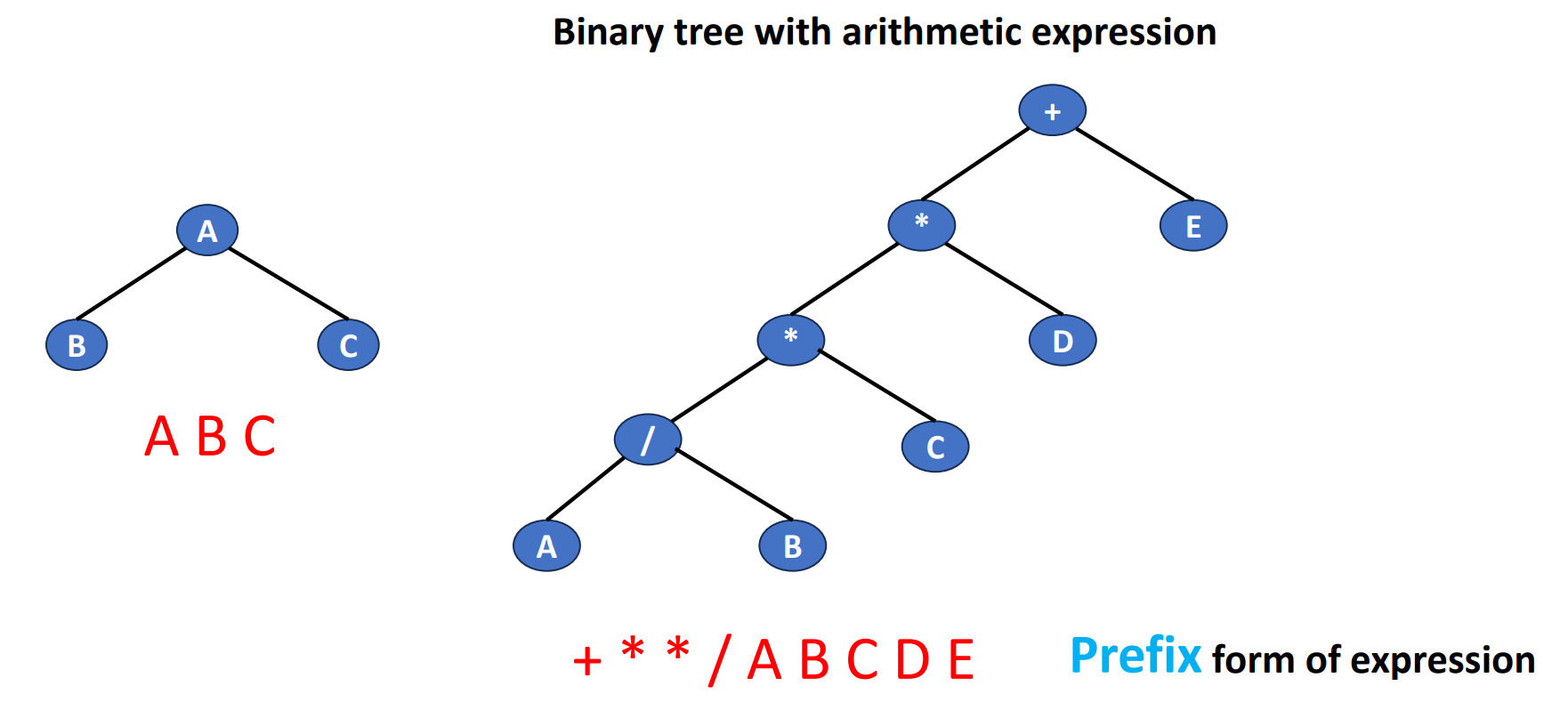
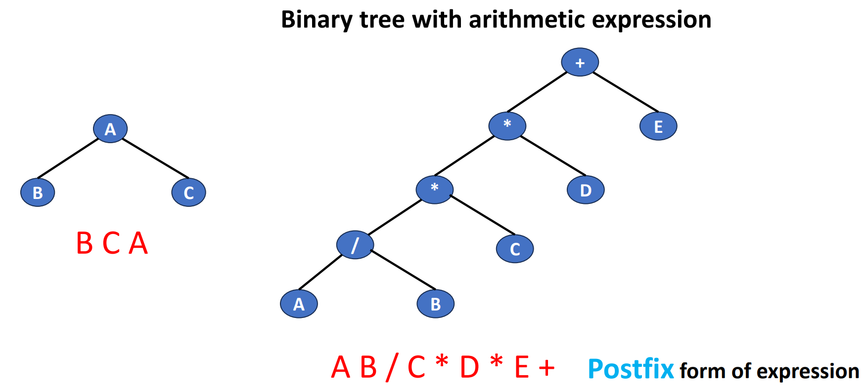
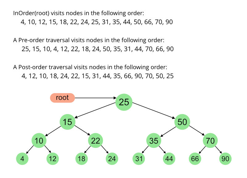
Binary Tree Traversal

Visiting each node in the tree exactly once
A traversal produces a linear order for the nodes in a tree
- LVR, LRV, VLR, VRL, RVL, and RLV
  - L
    - moving left
  - V
    - visiting the node
  - R
    - moving right
- LVR
  - Inorder
- VLR
  - Preorder
- LRV
  - Postorder

Inorder

void inOrder(treePointer ptr){
    if (ptr != NULL){
        inOrder(ptr->leftChild);
        visit(ptr);
        inOrder(ptr->rightChild);
    }
}

Preorder

void preOrder(treePointer ptr){
    if (ptr != NULL){
        visit(t);
        preOrder(ptr->leftChild);
        preOrder(ptr->rightChild);
    }
}

Postorder

void postOrder(treePointer ptr){
    if (ptr != NULL){
        postOrder(ptr->leftChild);
        postOrder(ptr->rightChild);
        visit(t);
    }
}

Difference Between Inorder, Preorder & Postorder

This is an illustration from GeeksforGeeks.

Level-Order

Visiting the nodes following the order of node numbering scheme (sequential numbering)

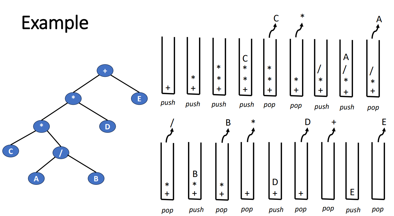
Iterative Traversal Using Stack

The following is an inorder example.

Push root into stack
Push the left into stack until reaching a null node
Pop the top node from the stack
- If there’s no node in stack, break
Push the right child of the pop-out node into stack
Go back to step 2 from the right child

Here’s the graph to let you more understand the workflow.

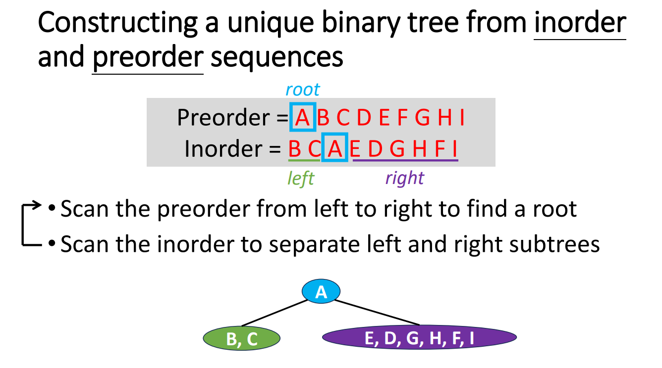
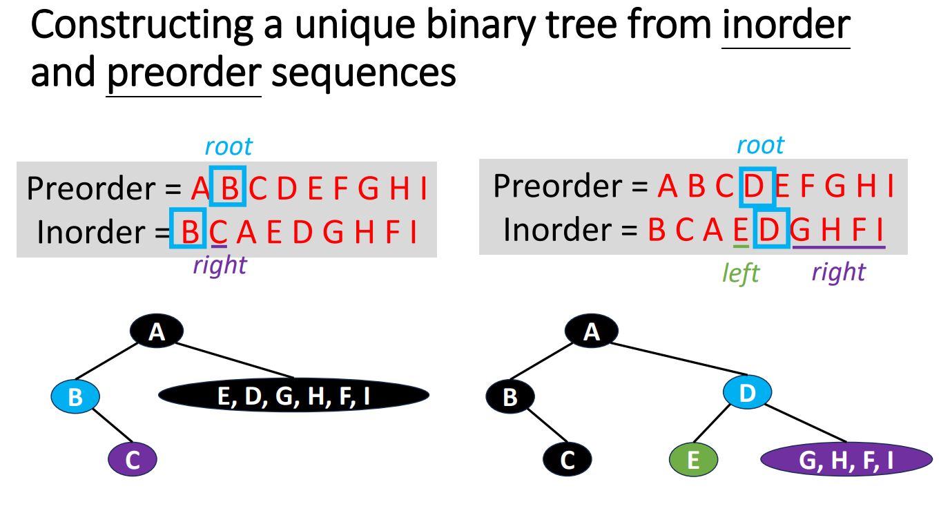
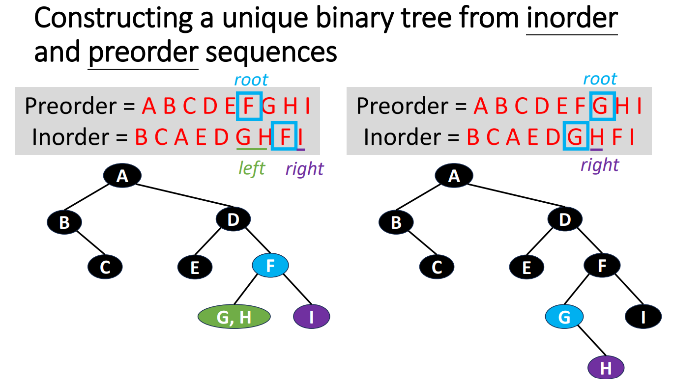
Convert Sequences Back to Trees

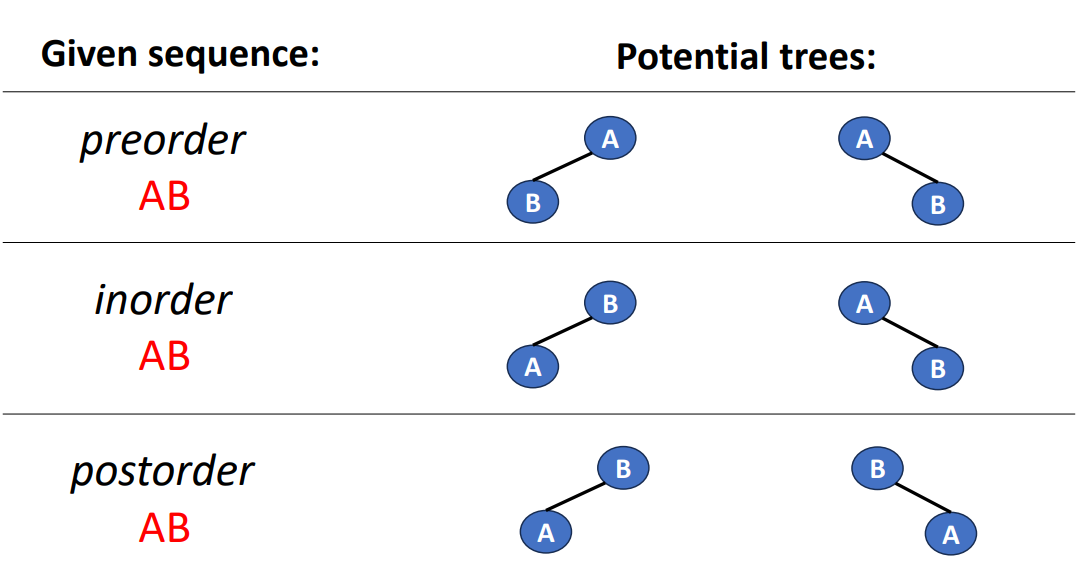
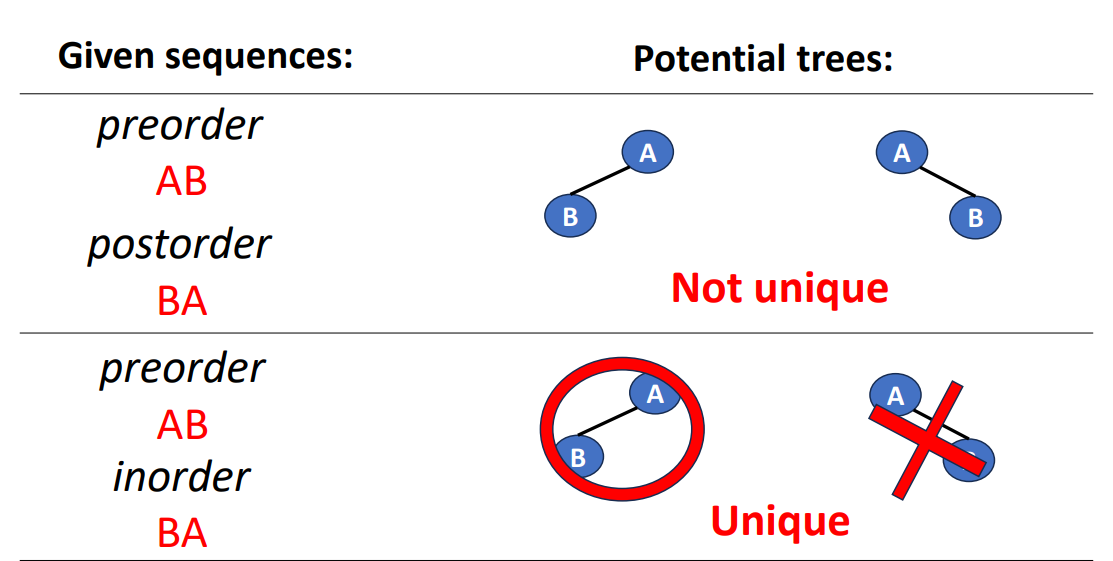
If we are given a sequence of data and we try to turn it back to a tree, how should we do? The following is an example of turnning a very short sequence data back into trees.

We can clearly see that if we are only given a sequence in 1 specific order, then we cannot know which side (left or right) is the original tree grows. But if we are given 2 different orders with 1 of them is inorder, then we can do it by the inference.

Binary Search Trees

Intro

The binary search tree, of course, it’s an binary tree. But beside this, it has some unique properties so that we can call it a binary search tree.

Each node has a (key, value) pair
Keys in the tree are distinct
For every node x
- all keys in the left subtree are smaller than that in x
- all keys in the right subtree are larger than that in x
The subtrees are also binary search tree.

Operations

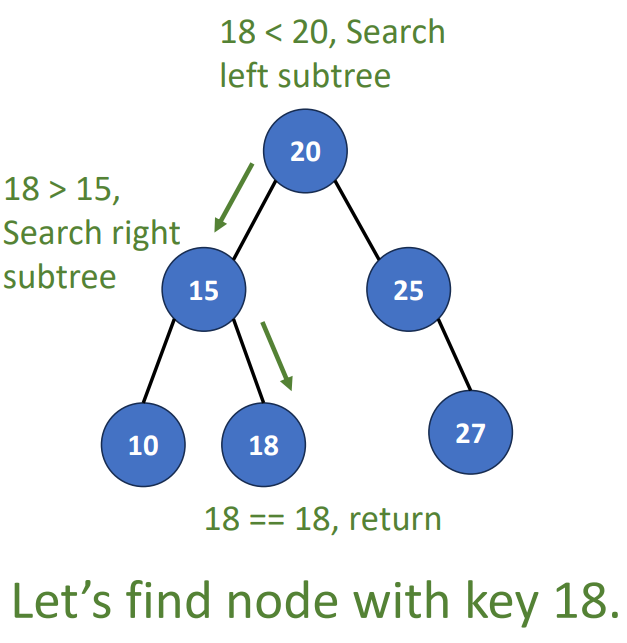
Search (root, key)

k == root’s key, terminate
k < root’s key, check left subtree
k > root’s key, check right subtree
Time complexity is $O(height)=O(n)$ , $n$ is number of nodes

Recursive

if (!root) return NULL;
if (k == root->data.key)
	return root->data;
if (k < root->data.key)
	return search(root->leftChild, k);
return search(root->rightChild,k)

Variable space requirement: $O(height) = O(n)$ , $n$ is the number of nodes.

Iterative

while(tree);
	if (k == tree->data.key)
		return tree->data;
	if (k < tree->data.key)
		tree = tree->leftChild;
	else
		tree = tree->rightChild;
return NULL

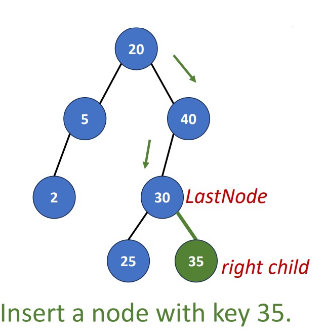
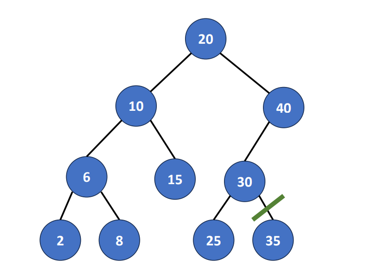
Insert(root, key, value)

Search the tree
- Matched: Do nothing
- No match: Obtain LastNode, which is the last node during the search.
Add new node
- Create a new node with (key, value)
- If key > the key of LastNode, add the new node as right child
- If key < the key of LastNode, add the new node as left child

Delete (key)

There’re 4 cases in the deletion.

No element with delete key
Element is a leaf
Element is a $degree-1$ node
Element is a $degree-2$ node

Since the 1st case means we don’t do anything, we will start from the 2nd case.

Delete a leaf

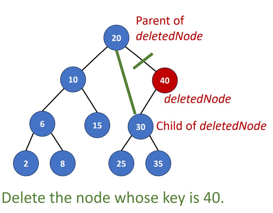
Delete a Degree-1 Node

Link the single child of the DeletedNode to the parent of DeletedNode.

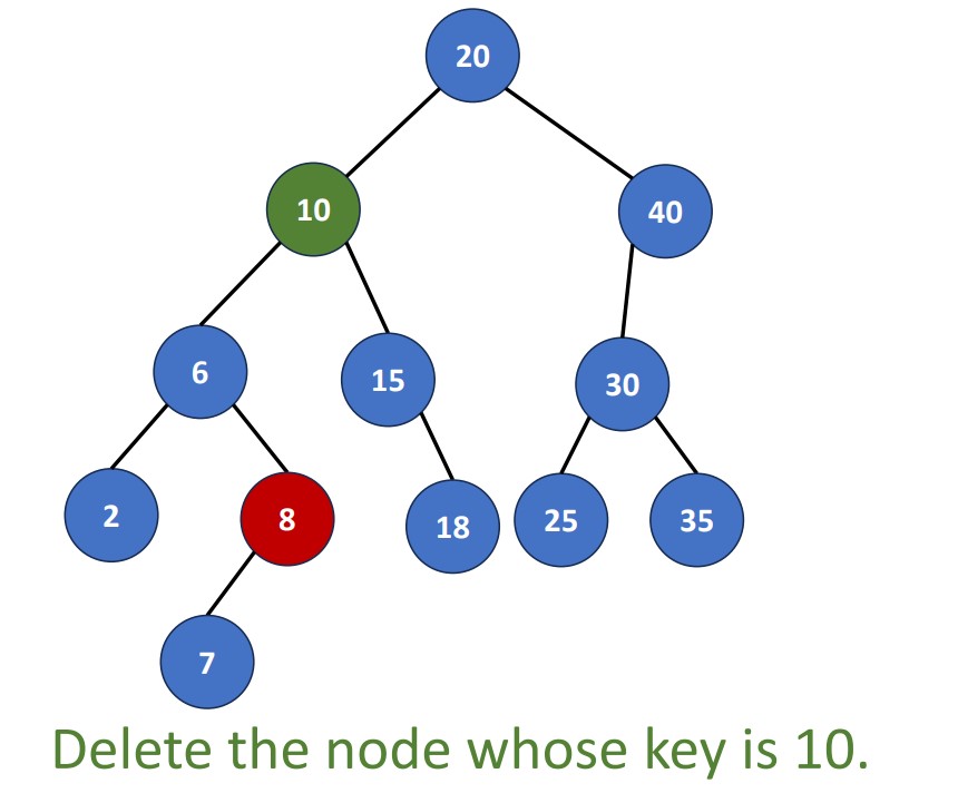
Delete a Degree-2 Node

There two ways to do it. We can replace the deleted node with

Largest pair in its left subtree
Smallest pair in its right subtree

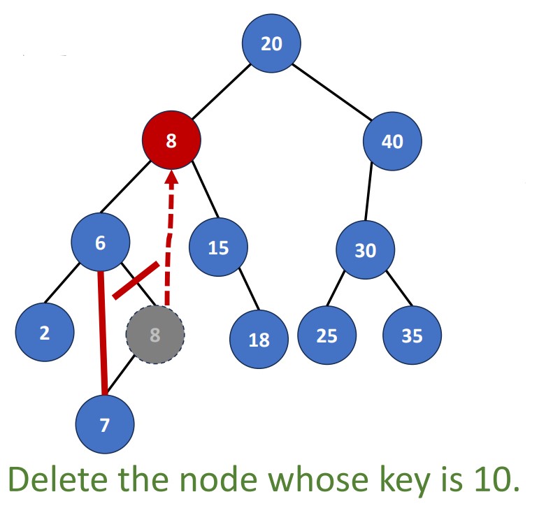
These two pairs must be leaf nodes or degree-one nodes. Why?

Rank of a Node in a BST

Rank of node $x$

The number of the nodes whose key values are smaller than $x$
Position of $x$ inorder
Like the index of an array

Heaps

Intro

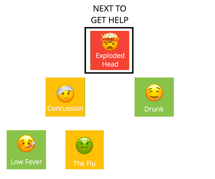
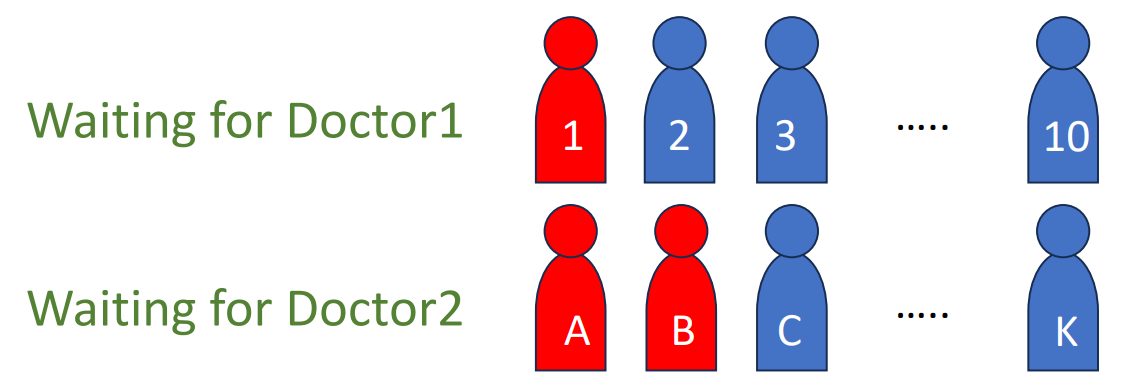
Imagine that we have a program that records patients waiting in the hospital, if the data structure we use is a queue (FIFO), and a dying person comes, we cannot let him queue up to see the doctor first.

So that’s why we need a priority queue! But how to implement one? Let’s dive into the heaps right away!

Min Tree & Max Tree

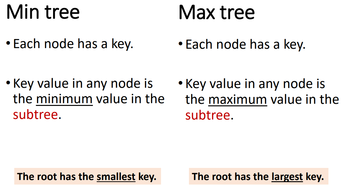
First, we should know what is min tree and max tree to establish the concept we will use later.

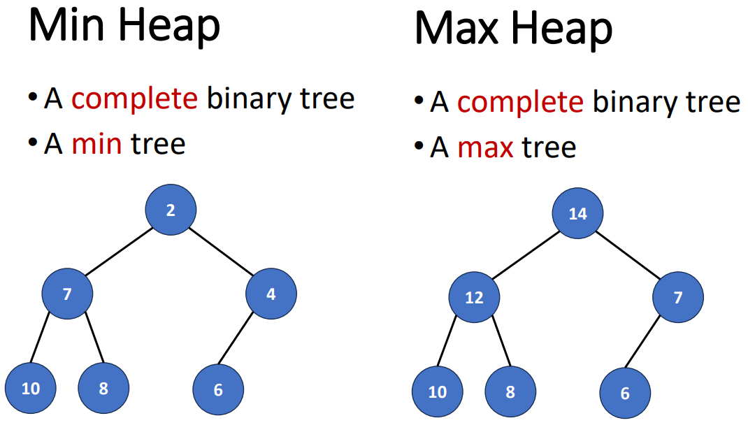
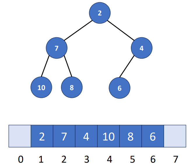
Min Heap & Max Heap

Array Representation

Operations

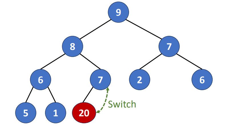
Here I use max heap for example, but it’s very similar with the min heap so you can try it by yourself! We’re going to use 2 operations called heapify up and heapify down.

Heapify up
- While the new element has a larger value than its parent, swap the new element and its parent
Heapify down
- While the “out of place element” has a smaller priority than any child, swap the out of place element with the smallest child

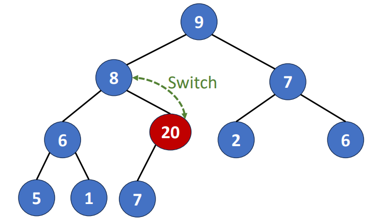
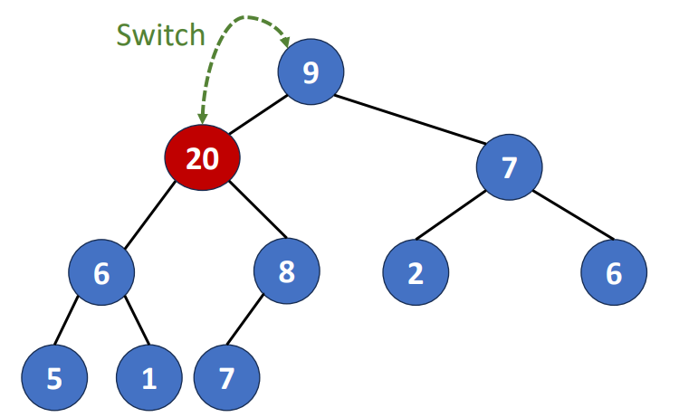
Insert(key)

Create a new node while keep the heap being a complete binary tree
Compare the key with the parent
- If the key < parent, pass
- If the key > parent, switch place with parent and recursively compare the parent with parent’s parent until it match the definition (key value in any node is the maximum value in the subtree)

This process is also called bubbling up process since it looks like a bubble goes up the water surface.

After we know how to insert things to a heap, we also care about it’s speed. The time complexity of the inseriton is $O(\log{n})$ , which $n$ is the heap size (height/level).

Delete() or Pop()

Removing the root of the heap
- Root is the min element in a min heap
- Root is the max element in a max heap

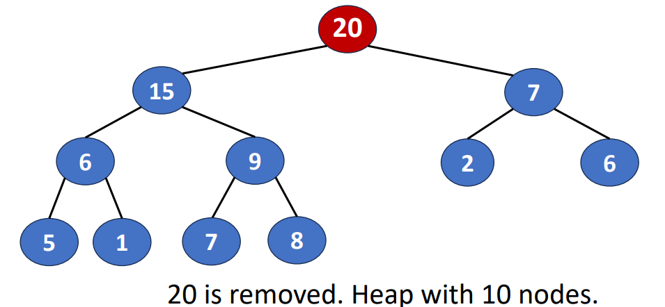
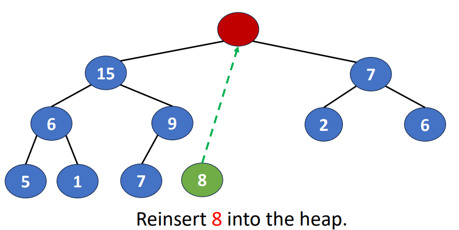
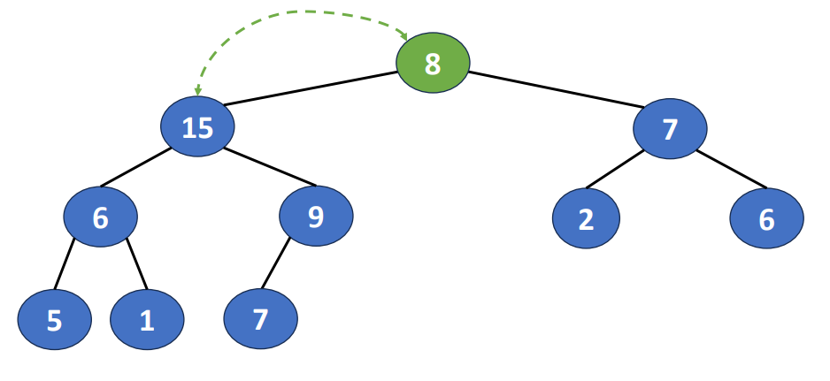
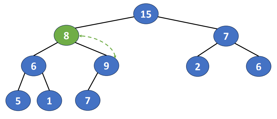
Following is the steps to do this operation

Removing the last node and inserting it into the root
Moving the node to a proper position
- Find the child containing max key value and exchange the position

And the time complextity of deletion is $O(\log{n})$ , where $n$ is also the heap size.

Leftist Heaps (Leftist Trees)

Intro

In previous part, we use the situation in hospital as an example to explain why we need priority queue, and now the situation becomes more complicated. In that hospital, 2 doctors are on call, just like the following graph.

But doctor1 becomes off duty, the 2 priority queues should be melded together for doctor2. To do this, we need the Leftist heaps!

Extended Binary Trees

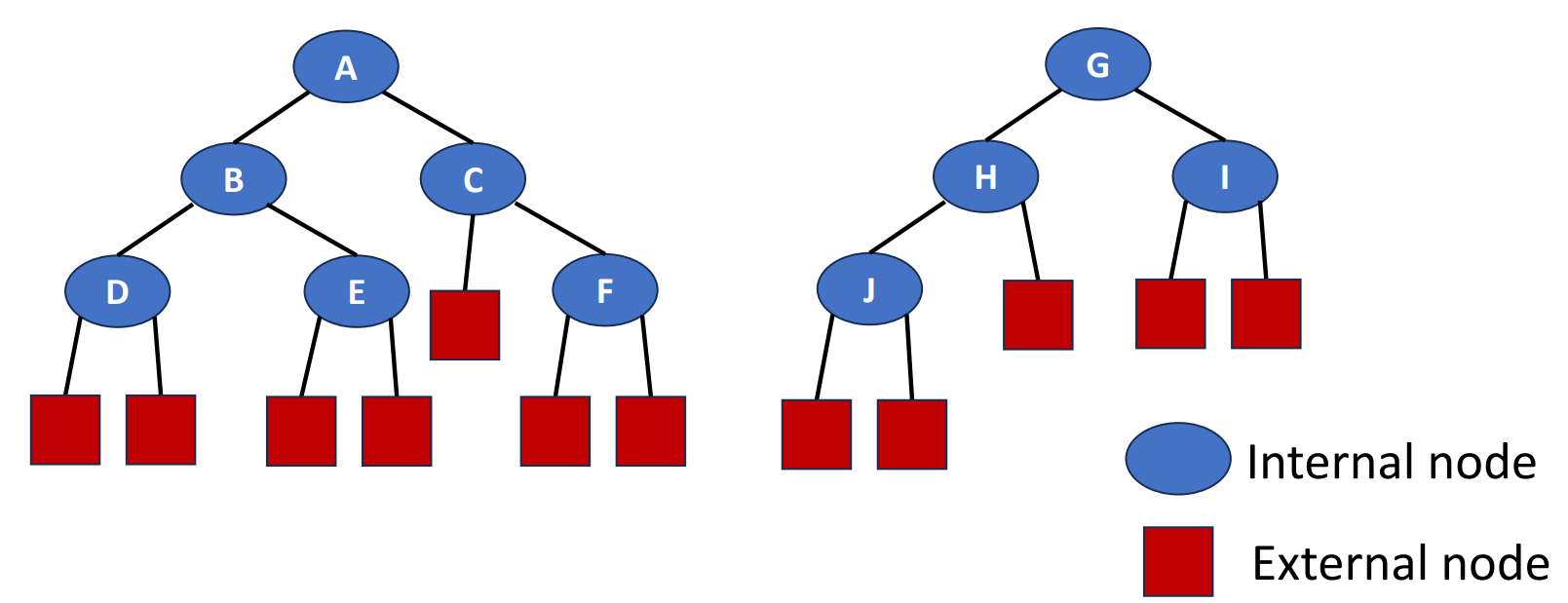
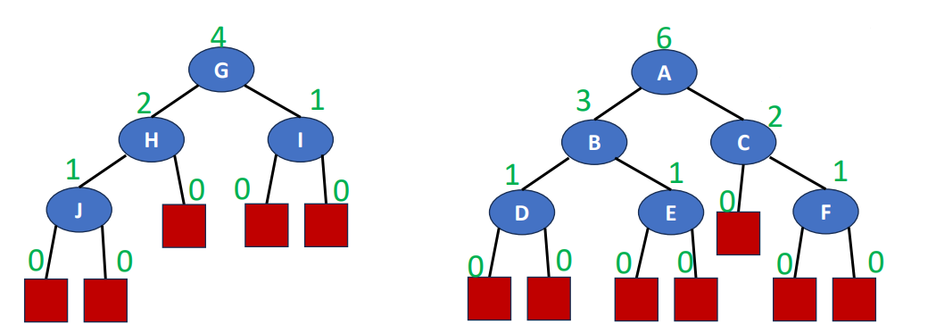
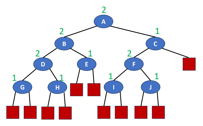
Before we step into the leftist tree, I need to introduce extended binary trees, a transformation of binary trees. To turn a binary tree into an extended binary tree, we just simply add an external node to every leaf in the original binary tree, then we obtained an extended binary tree! This is an example.

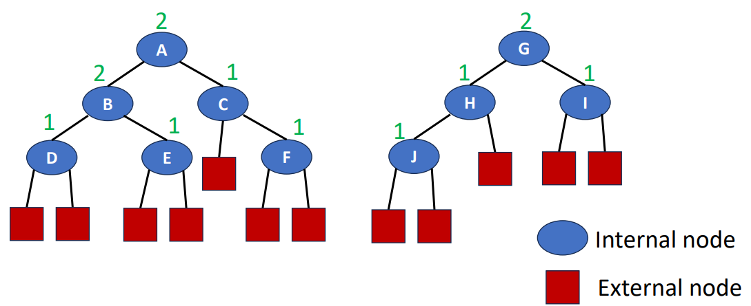
Function: Shortest(x)

Let’s say x is a node in an extended binary tree, then function shortest(x) is the length of a shortest path from x to an external node.

And here’s the formula for calculate the shortest(x) for all x belongs to internal nodes (since shortest(x) for all x in external nodes are 0).

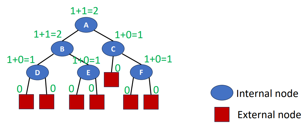
$shortest(x)=1+min(shortest(leftChild(x)), shortest(rightChild(x)))$

Function: Count(x)

This one will be a little easier to understand. Count means the nubmer of internal nodes. So for all x, which x is an internal node, we can calculate count(x) by the following formula (since count(x) of all x in external nodes are 0).

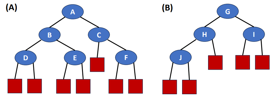
$count(x)=1+count(leftChild(x))+count(rightChild(x))$

Height-Biased Leftist Trees (HBLT)

Following is the definitioan of a HBLT:

An extended binary tree
For every internal node $x$ , $shortest(leftChild(x))\geq shortest(rightChild(x))$

In the following graph, B is a HBLT while A isn’t.

Weight-Biased Leftist Trees (WBLT)

Following is the definition of a WBLT:

An extended binary tree
For every internal node $x$ , $count(leftChild(x))\geq count(rightChild(x))$

In the following graph, the left is a WBLT while the right isn’t.

Properties of Leftist Trees

0x00

The rightmost path is a shortest from root to external node, that is shortest(root).

0x01

Number of internal nodes is $n\geq 2^{shortest(root)}-1$ .

That’s because the first shortest(root) level of nodes constitute a full binary tree, and for a shortest(root) level full binary tree, the total number of nodes is the following.

$\displaystyle\sum_{i=1}^{shortest(root)}2^{i-1}=2^{shortest(x)}-1$

And that’s why $n$ must be larger than $2^{shortest(root)}-1$ . Also, we can infer the following by this inequality.

$shortest(root)\le\log_2(n+1)$

0x02

Length of rightmost path is $O(\log n)$ , where $n$ is the number of nodes in a leftist tree.

Leftist Trees as Priority Queue

Remember the what I said in the first of this part? We need to make an priority queue that is easy to be merged with other one! Since we have learned min heaps and max heaps before, and leftist tree is actually a type of heap, we have the following types of leftist trees.

Min Leftist Tree
- Leftist tree that is a min tree. Used as a min priority queue.
Max Leftist Tree
- Leftist tree that is a max tree. Used as a max priority queue.

Operations

Given that the limited space, I will only use min leftist trees to be the examples, and all the operation here will be considered for min leftist trees. Nevertheless, they can all be applied to max leftist tree just by some modification.

Insert(x, T1)

Create a min leftist tree T2 containing only x
Merge T1 and T2

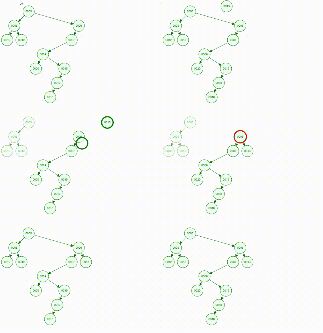
Following is the animation of inserting a 13 into a min leftist tree.

DeleteMin(T)

Get subtrees of root, T_left and T_right
Delete the original root
Merge T_left and T_right

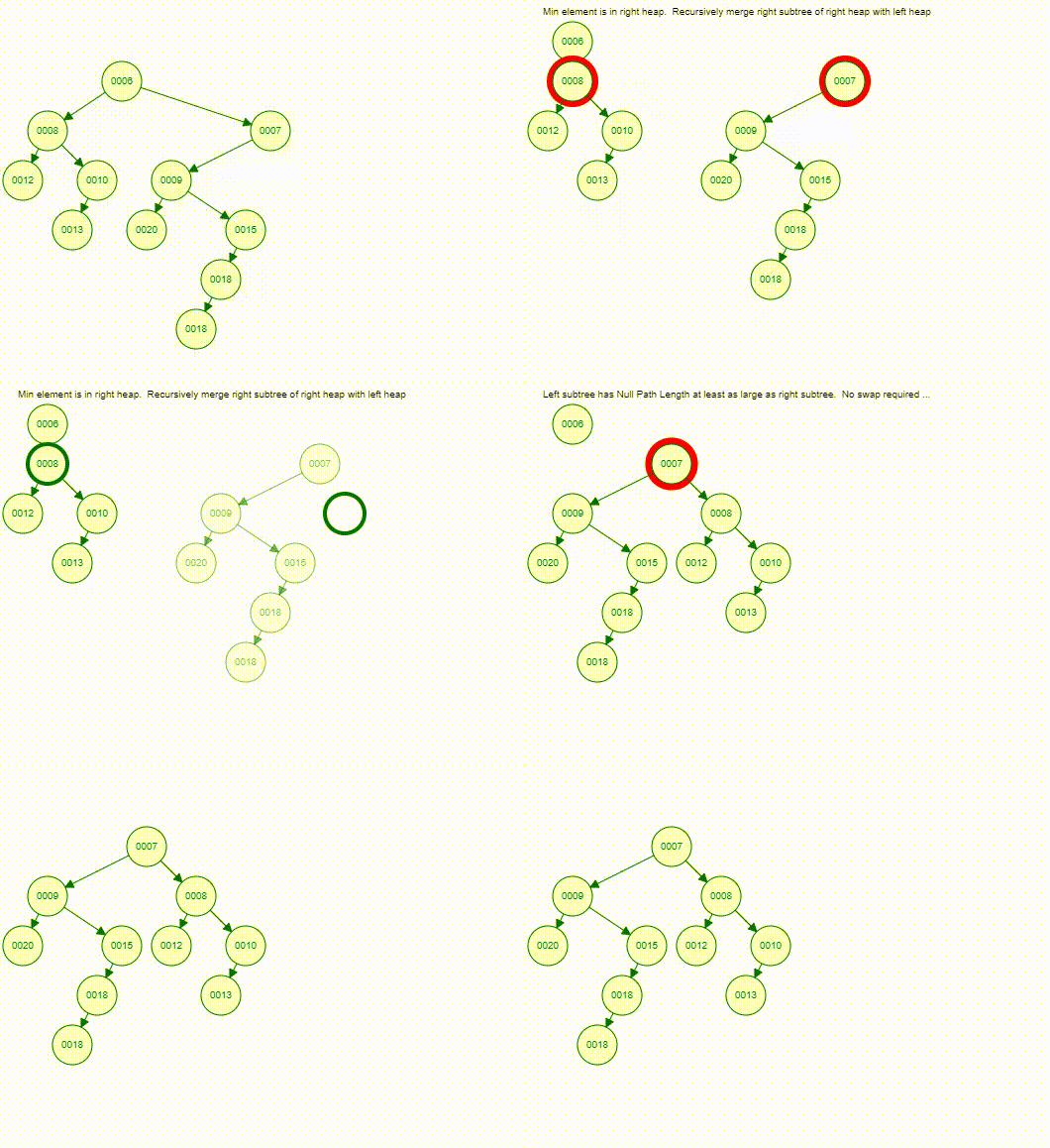
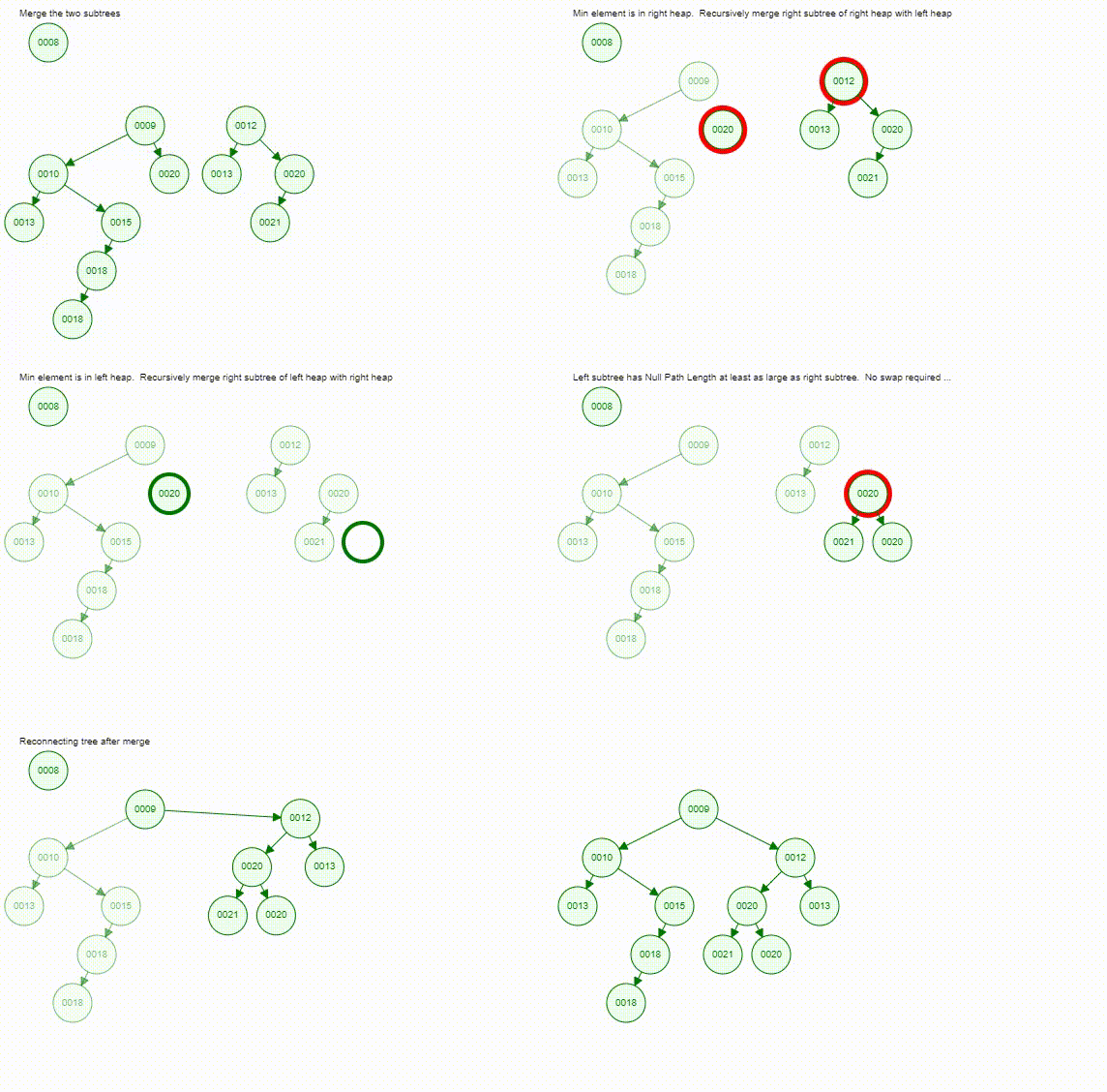
Following is the animation of deleting a minimum (6 in this case) from a min leftist tree.

Meld(T1, T2) or Merge(T1, T2)

Phase 1: Top-down process
- Maintaining the property of min tree
- Going down along the rightmost paths in T1 or T2 and comparing their roots
- For the tree with smaller root, going down to its right child
  - If no right child, attaching another tree as right subtree.
  - Else, comparing again
Phase 2: Bottom-up process
- Maintaining the property of leftist tree
- Climbing up through the rightmost path of the new tree
  - If not meet the definition of a leftist tree (HBLT or WBLT), interchange the left and right subtrees of the node
Time Complexity is $O(\log m)$ $O (lo g m)$
- Length of rightmost path is $O(\log n)$ , where $n$ is the number of nodes in a leftist tree
- A merge operation moves down and climbs up along the rightmost paths of the two leftist trees.
- $m$ is number of total elements in 2 leftist trees

The following is the animation of deleting a minimum from a min leftist tree, but please focus on the merge operation.

Initialize()

Create $n$ single node min leftist trees and place them in a FIFO queue
Repeatedly remove two min leftist trees from the FIFO queue, merge them, and put the resulting min leftist tree into the FIFO queue
The process terminates when only 1 min leftist tree remains in the FIFO queue
Time complexity is $n+2\times(1\times\frac{n}{2}+2\times\frac{n}{4}+3\times\frac{n}{8}+\dots)=O(n)$

Disjoint Sets

Intro

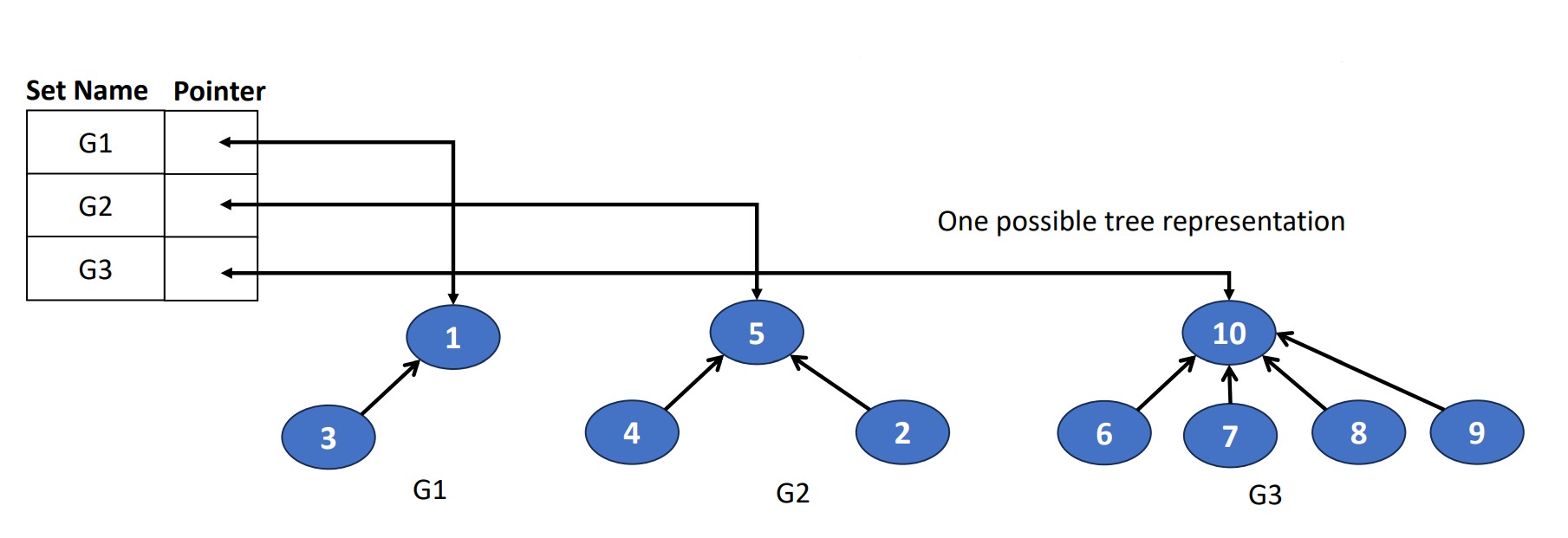
Let’s forget about the hospital scene, you are now a police officer. You know the relationship of 10 gangster, and No.1 & No.9 are suspects. How do you tell if they’re in a same gang? Let’s why we need disjoint sets! We can use this data structure to store the data like this.

There should Dbe no element appears in 2 different sets in the disjoint sets, which means a unique element should only appear once. Here are 2 examples.

$\begin{aligned} &S_1=\{0, 6, 7, 8\}\quad S_2=\{1, 4, 9\}\quad S_3=\{2, 3, 5\}\quad\text{Disjoint sets}\\ &S_1=\{0, 6, 7, 8, 9\}\quad S_2=\{0, 1, 4, 9\}\quad S_3=\{1, 2, 3, 5\}\quad\text{Not disjoint sets}\\ \end{aligned}$

Data Representation of Disjoint Sets

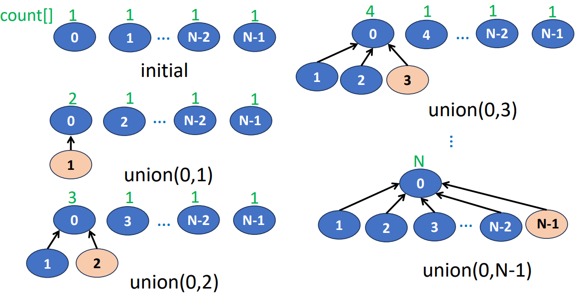
To represent a disjoint set, we link the node from the children to the parent, and each root has a pointer to the set name.

Operations

Find(i)

Find the set containing the targeted element
Start at the node representing element $i$ and climb up the tree until the root is reached. Then return the element in the root
Using an integer array to store the parent of each element
Time complexity depends on the level of $i$

while (parent[i] >= 0){
    i = parent[i]; // move up the tree
}
return i;

Union(i, j)

Combine 2 disjoint sets into 1
$i$ & $j$ are the roots of different trees, so $i\ne j$
For tree representation, we set the parent field of one root pointing to the other root
Which is making one tree as a subtree of the other. parent[j] = i
Time complexity is $O(1)$

$G_1=\{1, 3\}\quad G_2=\{6, 7, 8, 9, 10\}\quad G_3=G_1\cup G_2=\{1, 3, 6, 7, 8, 9, 10\}$

Sequence of Union-Find Operations

$\begin{aligned} &union(1, 0), find(0)\\ &union(2, 1), find(0)\\ &\quad\quad\quad\quad\vdots \\ &union(N-1, N-2), find(0) \end{aligned}$

For each find(0), we trace from 0 to the root.

Time complexity
- Time to initailize parent[i] = 0 for all elements is $O(n)$
- $n-1$ times of union(), each time takes $O(1)$ , so total is $O(n)$
- $n-1$ times of find(), each time takes $i$ , so total is $\displaystyle\sum^n_{i=2}i=O(n^2)$

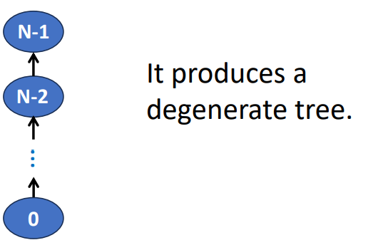
How to avoid the creation of degenerate tree? Let’s see in next part of this chapter!

Weight Rule for Union(i, j)

Make tree with fewer number of elements a subtree of the other tree
The count of the new tree is the sum of the counts of the trees that are united

Height Rule for Union(i, j)

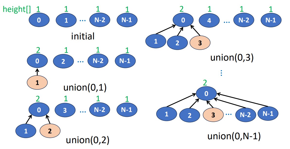
Make tree with smaller height a subtree of the other tree
The height increases only when two trees of equal height are united

Collapsing Rule

Lemma 1

Suppose we start with single element trees and perform unions using either the height rule or the weight rule
The height of a tree with $p$ element is at most $floor(\log_2p)+1$
Processing an intermixed sequence of $u-1$ unions and $f$ finds, the time complexity will be $O(u+f\log u)$
$u-1$ unions part, we generate a tree with $u$ nodes
$f$ finds part, it requires at most $f\times[floor(\log_2u)+1]$

Improving Find(i) with Collapsing Rule

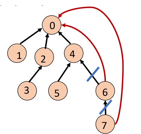
Collapsing rule means:

Make all nodes on find path point to tree root
Pay some more efforts this time, but the Find() operations in the future could save time
Slower this time, faster next time

Here’s an example, if we have a sequence $find(7),find(7),find(7),find(7),find(7)$ to this tree.

Without collapsing rule
- A $find(7)$ requires climbing up 3 times
- Total is $5\times 3=15$ moves
With collapsing rule
- The first $find(7)$ requires climbing up 3 times
- The remainding $find(7)$ only needs to climbing up once
- Total is $3+4\times 1=7$ moves

Lemma 2 (By Tarjan and Van Leeuwen)

Let $T(f, u)$ be the maximum time required to process any intermixed sequence of $f$ finds and $u$ unions. Assuming that $u\geq\frac{n}{2}$

$k_1\times(n+f\times\alpha(f+n,n))\le T(f,u)\le k_2\times(n, f\times\alpha(f+n,n))$

where $k_1$ and $k_2$ are constants, $n$ is the number of elements, and $\alpha(f+n, n)$ is inverse Ackermann function.

Ackermann function
- A function of 2 parameters whose value grows very, very fast
Inverse Ackermann function
- A function of 2 parameters whose value grows very, very slow

Time Complexity

Those bounds in Lemma 2 can be applied when we start with singleton sets and use either the weight or height rule for unions and collapsing rule for a find. The time complexity will be $O(n+f)$ , which is very efficient.

Graphs

Intro

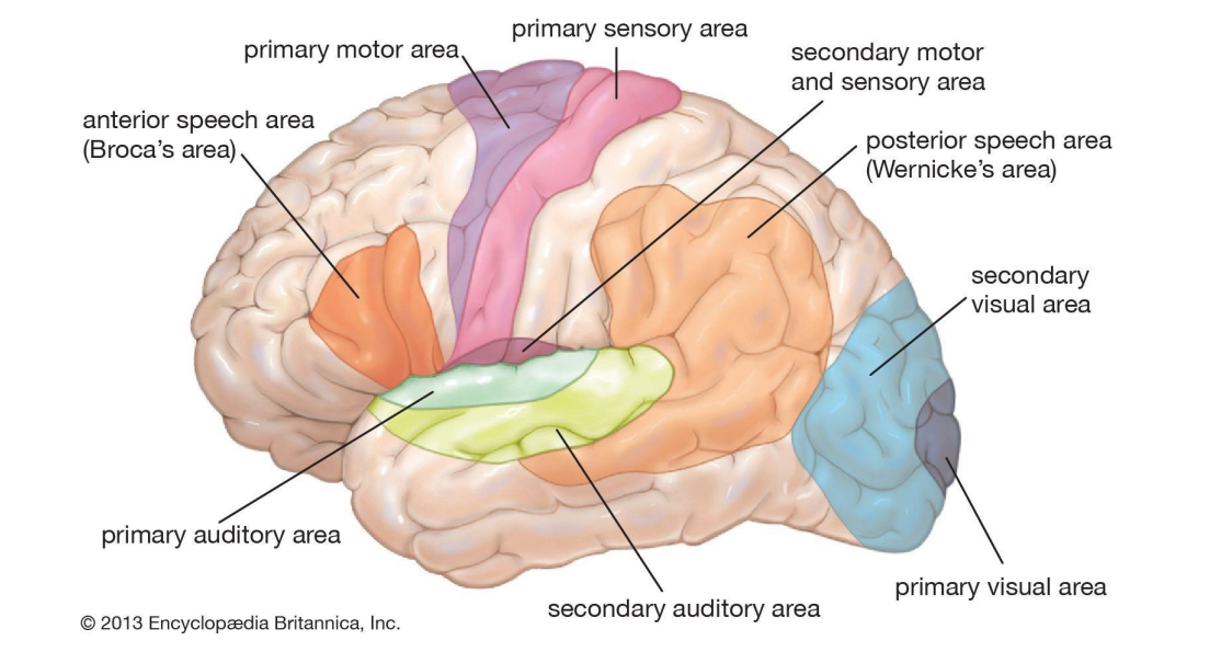
Now, let’s talk about the brains of the humanities. In out brain, each region is associated with different functions. Just like the graph below.

But the works in reality are complicated, so we usually use multi-part of out brain to achieve a task. That’s what we can represented by a graph. It will be easier for us to visualize and further analysis.

Graph can be represented as this form.

$G=(V, E)$

$V$ $V$ : Set of vertices
- Vertices are also called nodes or points
$E$ $E$ : Set of edges
- Each edges connected 2 different vertices
- Edges are also called arcs & lines
- In undirected graph, $(u, v)$ and $(v, u)$ represent the same edge
- In directed graph, $<u, v>$ and $<v, u>$ represent different edges

With graph, we can do a lot of applications, such as planning a route from city A to city B, witch we can let vertices to be cities, edges to be roads and edge weight to be the distances or times we need. Now, let’s go to the next part and know more terms of graph.

Terminology

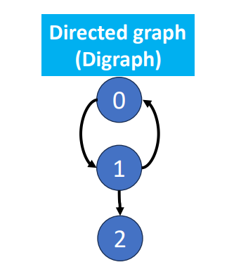
Directed Graph

There’ direction between the connections of the vertices.

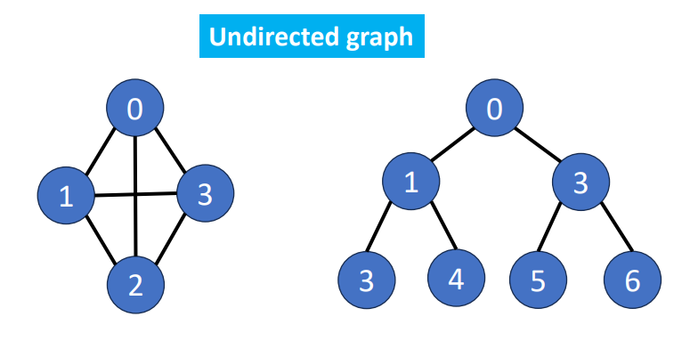
Undirected Graph

There’s no direction between the connections.

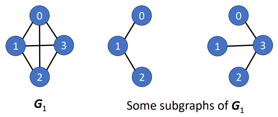
Subgraph

A graph that is composed of a subset of vertices and a subset of edges from another graph.

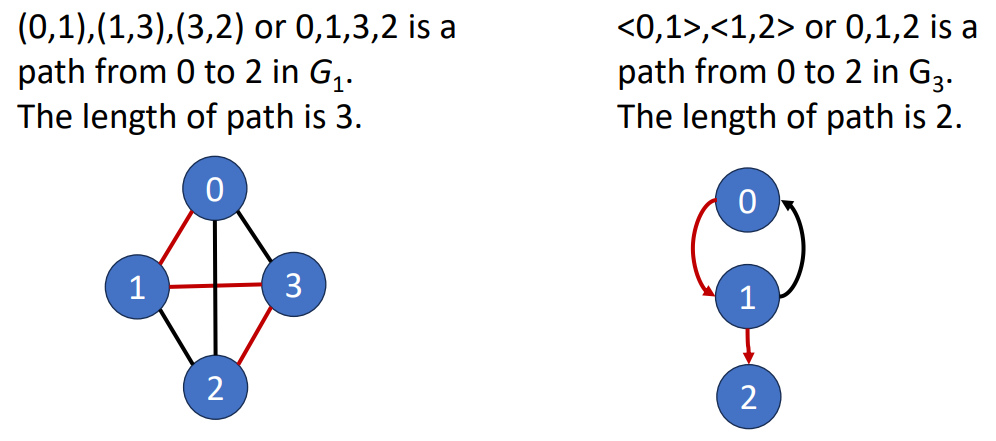
Path

Length of a path is the number of edges on it.

Simple Path & Cycle

SImple Path
- No repeating vertices (except for the case that the first and the last are the same)
Cycle
- Simple path
- The first and the last vertices are the same

$\begin{aligned} &0, 1, 3, 2\quad\text{Simple path}\\ &0, 1, 3, 1\quad\text{Not simple path}\\ &0, 1, 2, 0\quad\text{Cycle} \end{aligned}$

Connection

2 vertices $u$ and $v$ are connected if and only if there’s a path from $u$ to $v$
Connected component
- A maximum subgraph that are connected to each other
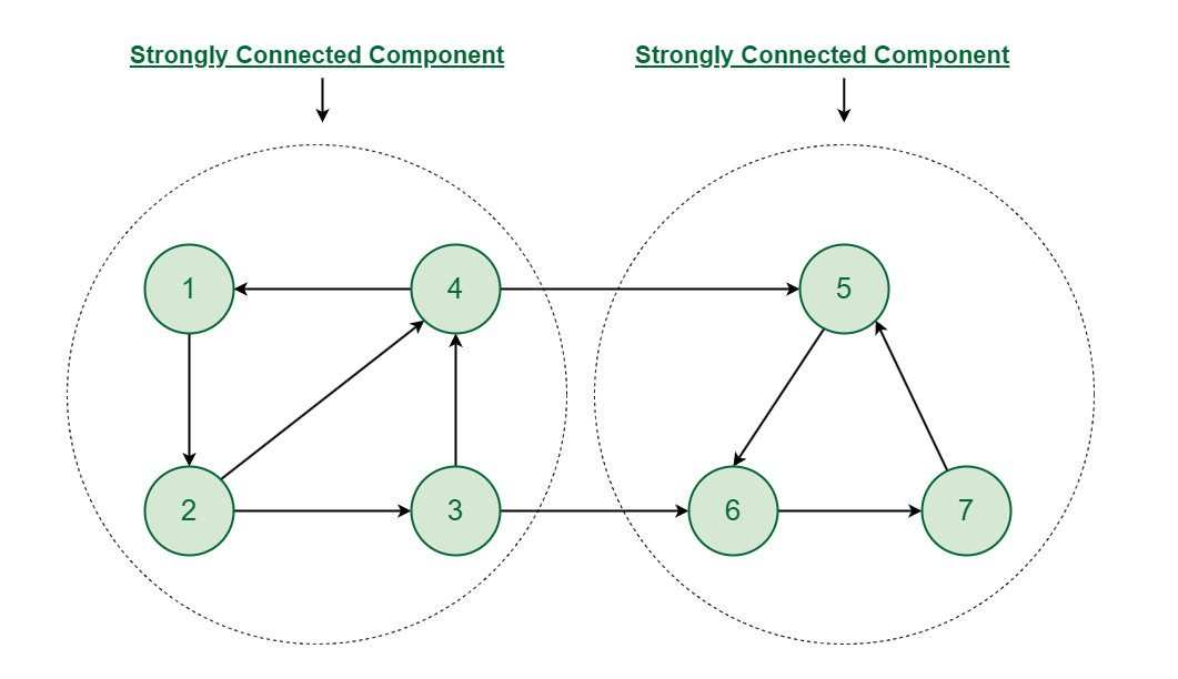
Strongly connected component
- In a direct graph, every pair of vertices $u$ and $v$ has a directed path from $u$ to $v$ and also from $v$ to $u$

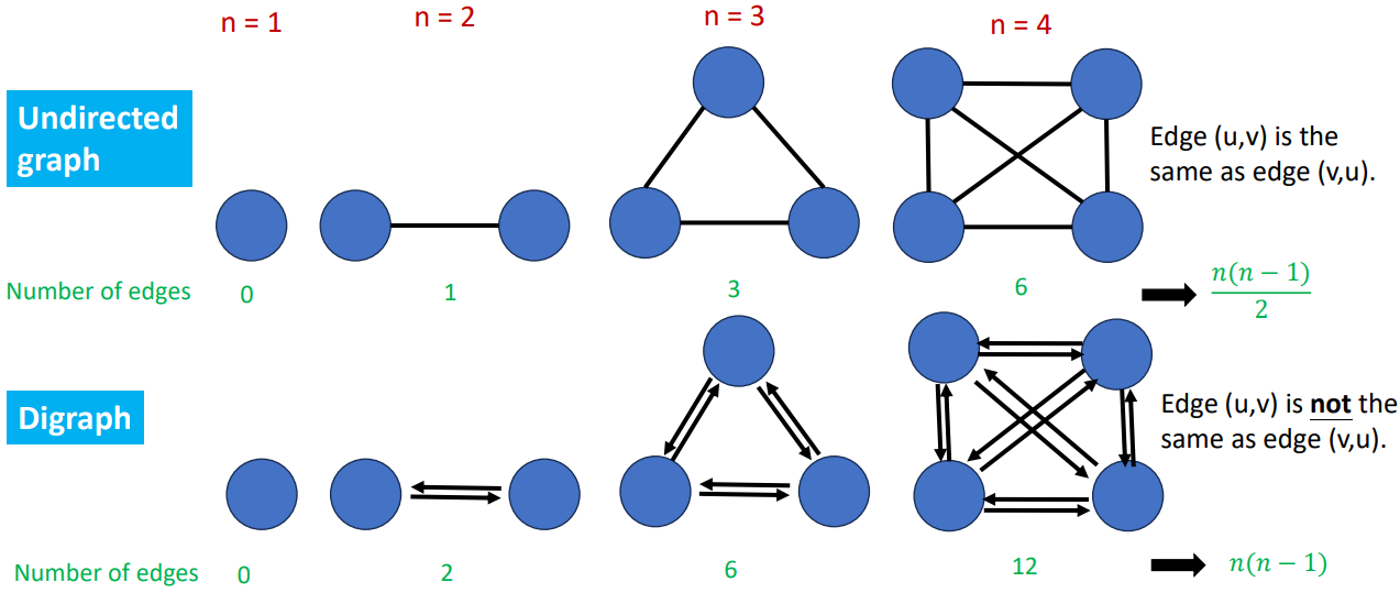
Complete Graph

Having the maximum number of edges

Properties

Number of Edges

If we set $n$ to be the number of vertices and $e$ to be the number of edges, then

Undirected Graph
- $e\le n(n-1)/2$
Directed Graph
- $e\le n(n-1)$

Vertex Degree

Number of edges incident to vertex
Directed graph
- In-degree, which is pointed into the vertex
- Out-degree, vice versa

Sum of degree

The number of edges is $e$ , then

Undirected Graph
- $2e$
- Since each edges contributes $2$ to vertex degree
Directed Graph
- $e=sum(in)=sum(out)$

Trees & Spanning Trees

Tree

Acycilc Graph
- A graph with no cycles
Connected Graph
- All pairs of nodes are connected
- $n$ vertices connected graph with $n-1$ edges

Spanning Tree

A tree
A subgraph that includes all vertices of the original graph
If the original graph has $n$ vertices, then the spanning tree will have $n$ vertices and $n-1$ edges

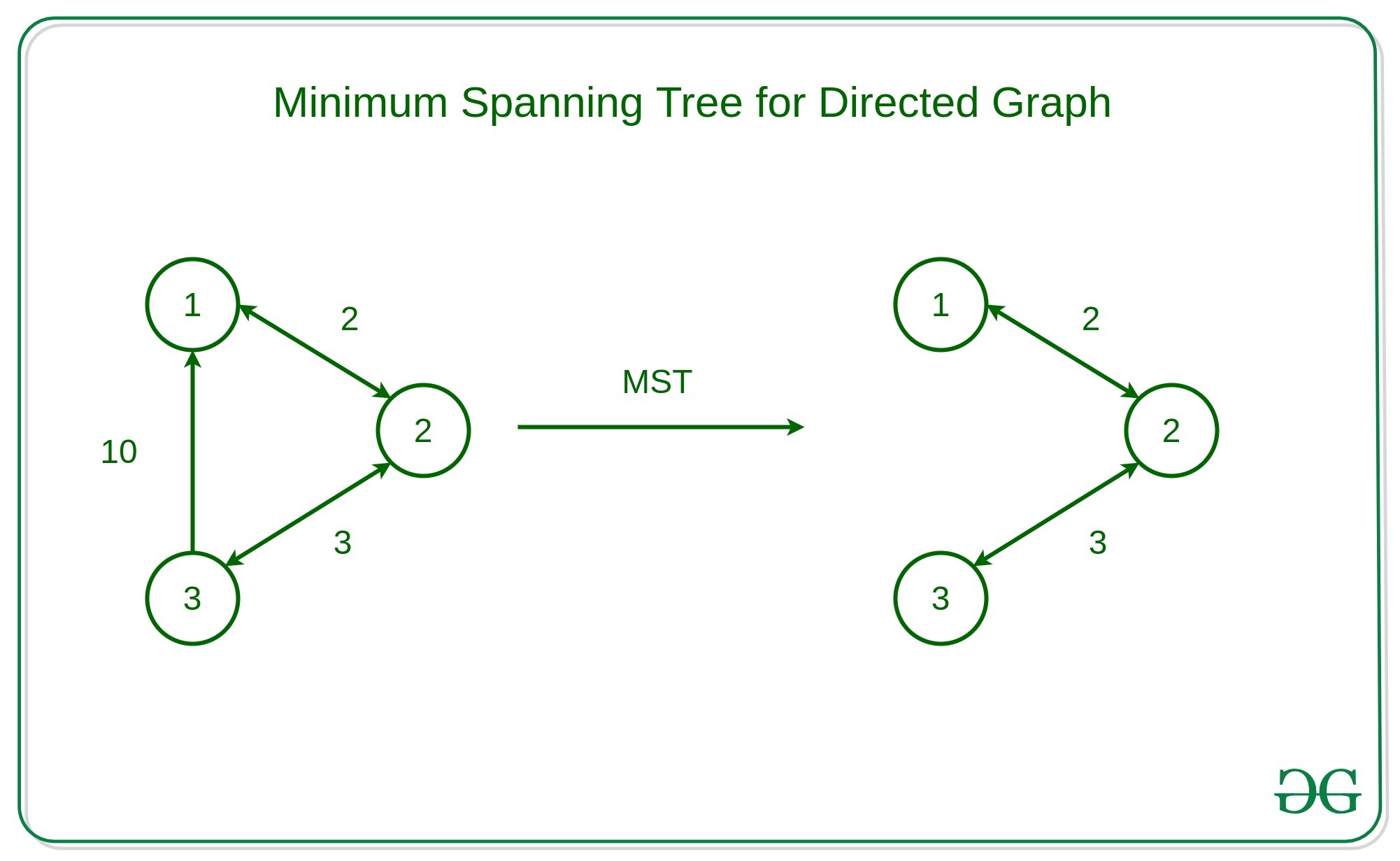
Minimum Cost Spanning Tree

A spanning tree with least cost (or weight)
- Tree cost means the sum of edge costs/weights

Graph Representaions

Adjacency Matrix

Using 2-Dimensional $n$ $n$ by $n$ $n$ matrix $A$ $A$
- $n$ is number of vertices
- $A[i][j]=1$ means there to be an edge between vertices $i$ and $j$
- Diagonal entries are all $0$

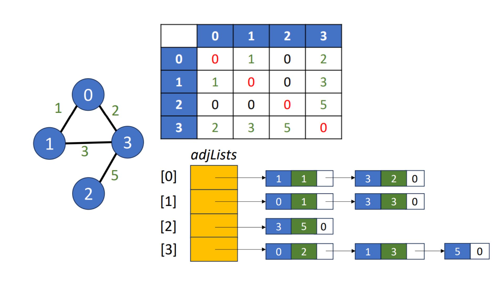
Traversing this matrix will have the time complexity $O(n^2)$ , it seems to be okay in a small matrix. But what if the matrix is large and sparse? There’s only a little 1s in the matrix, which are the things we care (cause we don’t care about the zeros), how can we improve the time complexity? We can use other ways to represent an graph.

Linked Adjacency List

Undirected Graph

Each adjacency list is a chain. One chain for each vertex
- Array length will be $n$
The data field of a chain node store an adjacency vertex
- In undirected graph, total number of chain nodes will be $2e$

Directed Graph

Total nubmer of chain nodes is $e$
The data field of a chain node store an adjacent vertex
In inverse linked adjacency list, the data field of a chain node store the vertex adjacent to the vetex it represents

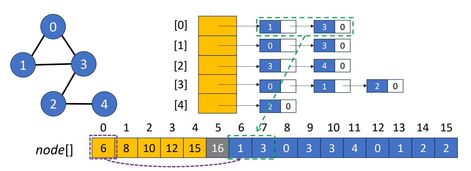
Array Adjacency List

Using an integer array node[] to store all adjacency lists
- Array length will be $n+2e+1$
- The $i^\text{th}$ element in node[0, 1, 2, ..., n-1] is the starting point of the list for vertex $i$

Weighted Graphs

Weighted adjacency matrix
- $A[i][j]$ is cost of edge $(i, j)$
Weighted adjacency list
- Each element is a pair of adjacent vertex & edge weight
A graph with weighted edges is called a network

DFS & BFS

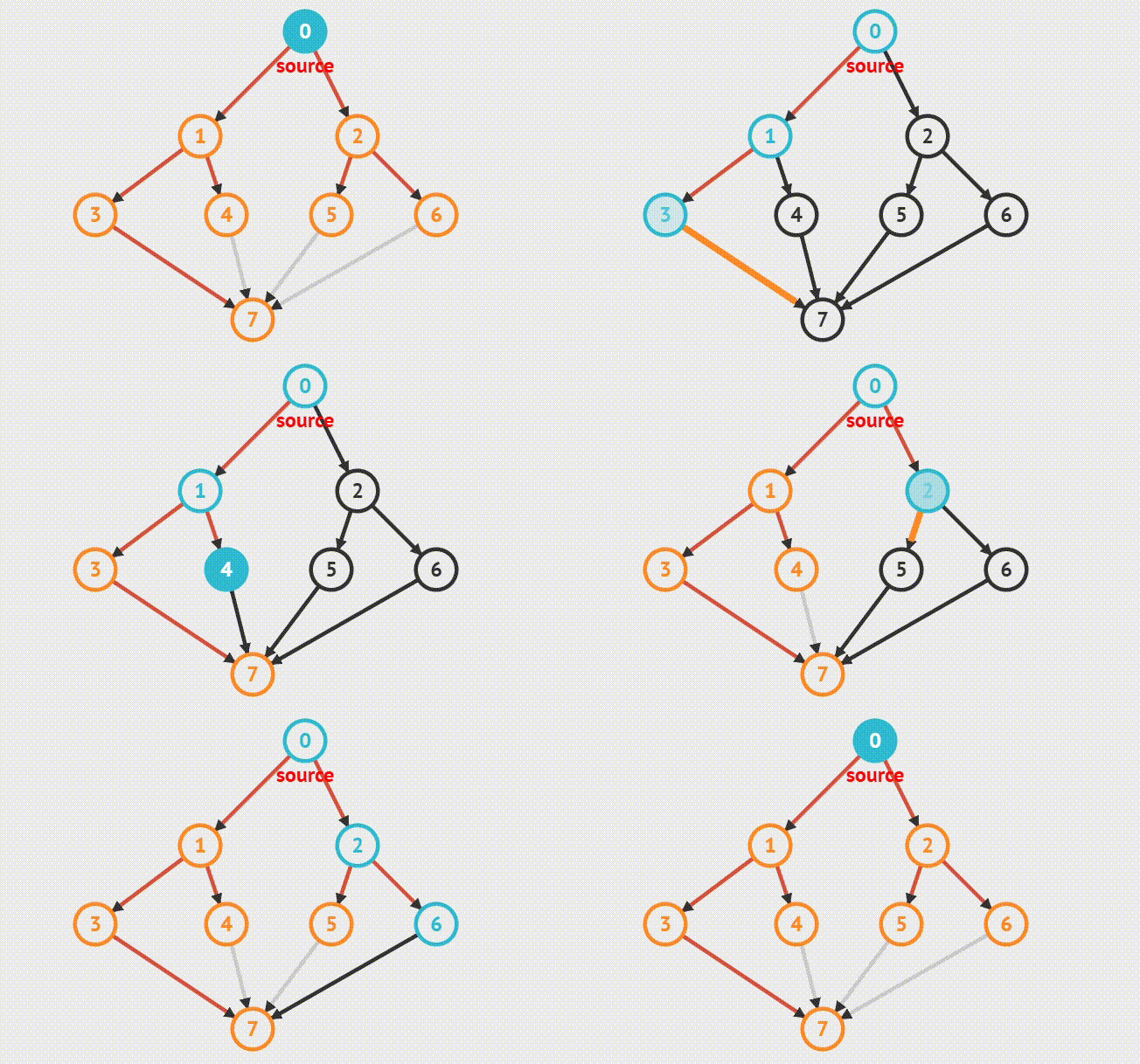
To search element in a graph, we need to introduce 2 algorithms, depth first search and breadth first search.

Depth First Search (DFS)
- Similar to a preorder tree traversal
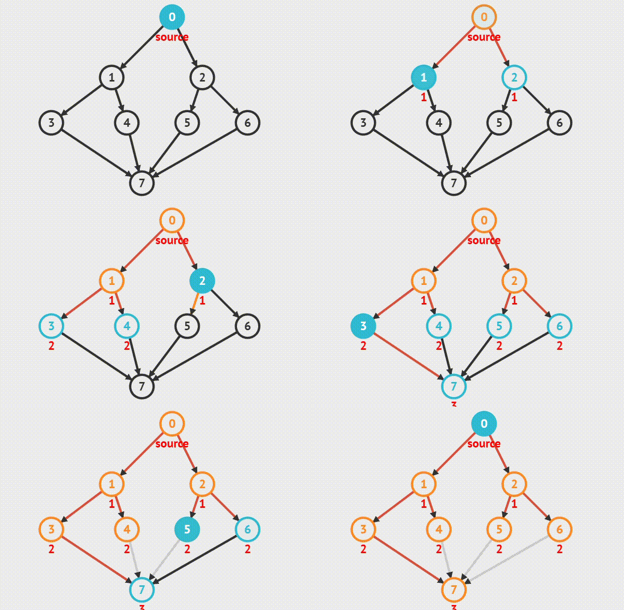
Breadth First Search (BFS)
- Similar to a level-order tree traversal

If there’s a path from a vertex $u$ to another vertex $v$ , we say $v$ is reachable from $u$ . A search method is to traverse/visit every reachable vertices in the graph.

DFS

Here’s the pseudo code and animation of DFS.

short int visited[MAX_VERTICES];
/*Depth first search of a graph beginning at v.*/
dfs(v){
    /*Label vertex v as reached.*/
    visited[v] = TRUE;
    /*Explore the adjacent unvisited vertices.*/
    for (each unreached vertex u adjacent from v)
    dfs(u);
}

BFS

Visit start vertex and put into a FIFO queue
Repeatedly remove a vertex from the queue, visit its unvisited adjacent vertices, put newly visited vertices into the queue

Here’s the pseudo code and animation of BFS.

// From VisuAlgo
BFS(u), Q = {u}

while !Q.empty // Q is a normal queue (FIFO)

    for each neighbor v of u = Q.front, Q.pop

        if v is unvisited, tree edge, Q.push(v)

        else if v is visited, we ignore this edge

Time Complexity

Adjacency matrix, the time complexity is $O(n^2)$ $O (n^{2})$
- For each node, searching the corresponding row to find adjacent vertices takes $O(n)$
- Visiting at most $n$ nodes takes $O(n\times n)=O(n^2)$
Adjacency list, the time complexity is $O(n+e)$ $O (n + e)$
- Search at most $e$ edges and $n$ nodes

Application: Articulation Points

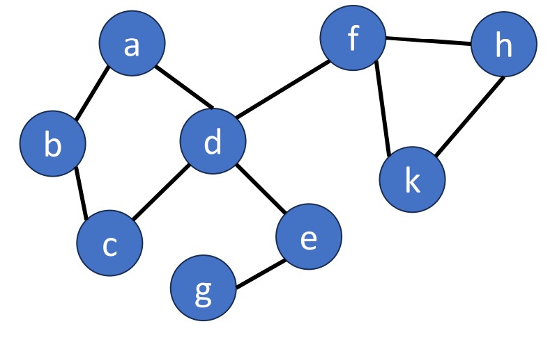
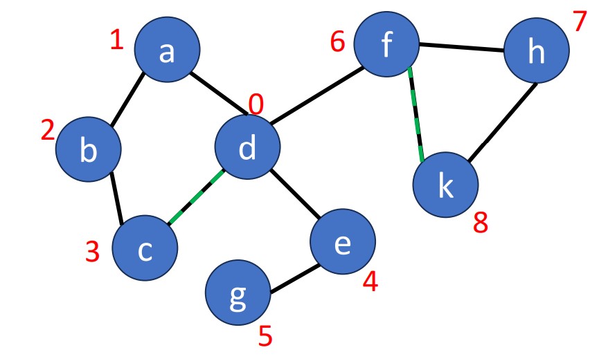
Articulation Point means if a vertex is deleted, at least 2 connected components are produced, then the vertex is called articulation point. In the graph below, $d$ and $f$ are articulation points, for example.

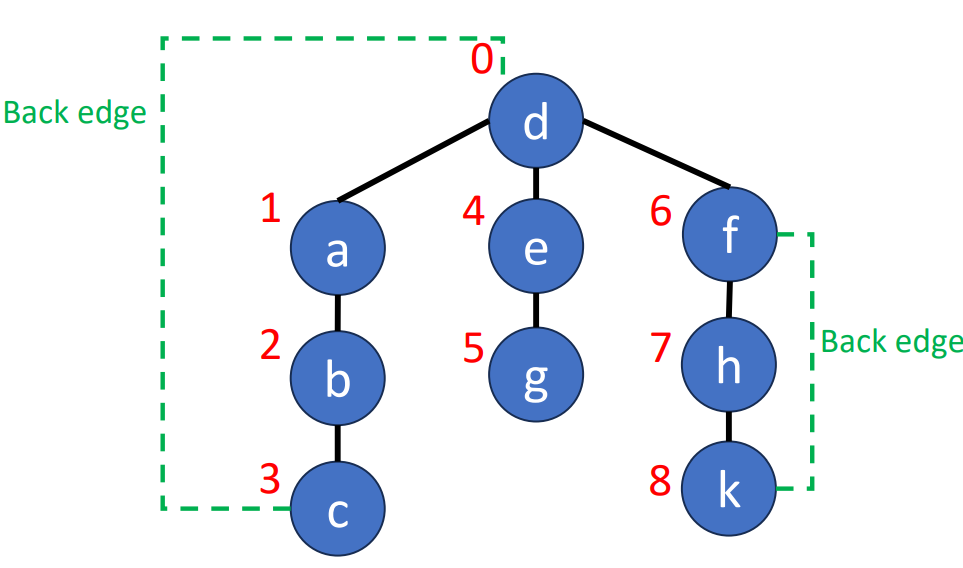
To find a articulation point, we can generate a depth-first search spanning tree. Using the graph above as an example, we use dfs(d) to generate a spanning tree.

For root $r$ $r$
- $Degree(r)\ge2$ , then $r$ is an articulation point
For a non-root vertex $v$ $v$
- A child of vertex $v$ cannot reach any ancestor of vertex $v$ via other paths, then $v$ is an articulation point

Minimum Spanning Trees (MST)

Intro

In a weighted connected undirected graph $G$ $G$
- $n$ is number of vertices
A spanning tree of the least weights
- Weights/Costs is the sum of the weights of edges in the spanning tree
- Edges within the graph $G$
- Number of edges is $n-1$

How can we derive an MST from a graph?

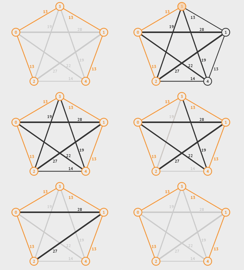
Kruskal’s Method

Start with an forest composed of $n$ vertices and $0$ edges
Select edges in nondecreasing order of weight
- If not form a cycle with the edges that are already selected

Pseudo Code

T = {};
while (|T| < N-1 and E is not empty){
    choose a least cost edge (v,w) from E;
    E = E – {(v,w)}; /*delete edge from E*/
    if (adding (v,w) doesn’t create a cycle in T)
    T = T + {(v,w)}; /*add edge to T*/
}
if (|T| == N – 1) T is a minimum cost spanning tree.
else There is no spanning tree.

Data Structures for Kruskal’s Method

Operations related to $E$ $E$
- Check if the edge set $E$ is empty
- Select and remove a least-weight edge
- Use a min heap or leftist heap for edges set
- Time complexity
  - Initialization: $O(e)$
  - Remove and return least-weight edge: $O(\log e)$
Operations related to $T$ $T$
- Check if $T$ has $n-1$ edges
- Examine if adding $(u, v)$ $(u, v)$ to $T$ $T$ creates a cycle
  - Each connected component in $T$ is a set containing the vertices, like $\{a, g\},\{f\}, \{h, b, c, e\}$
  - Adding 2 vertices that are already connected creates a cycle
  - Using find() operation to determine if $u$ and $v$ are in the same set
- Add an edge $(u, v)$ $(u, v)$ to $T$ $T$
  - If an edge $(u, v)$ is added to $T$ , the 2 connected components that have vertices $u$ and $v$ should be merged
  - Using union() operation to merge the set containing $u$ and $v$
  - $\{f\}+\{h, b, c, e\}=\{f, h, b, c, e\}$
- Use disjoint sets to process $T$

Time Complexity

Operations for edge set $E$ $E$
- Initialize min heap or leftist heap: $O(e)$
- Operations to get minimum weight edge: $O(\log e)$ $O (lo g e)$
  - At most $e$ times of operation: $O(e\log e)$
Operations for vertices
- Initialize disjoint sets: $O(n)$
- At most $2e$ find operations and $n-1$ union operations: close to $O(e+n)$
Overall: $O(e+e\log e+n+e)\approx O(e\log e)$ $O (e + e lo g e + n + e) \approx O (e lo g e)$
- For each iteration, time for union-find operation is less than that for obtaining minimum cost edge

Prim’s Method

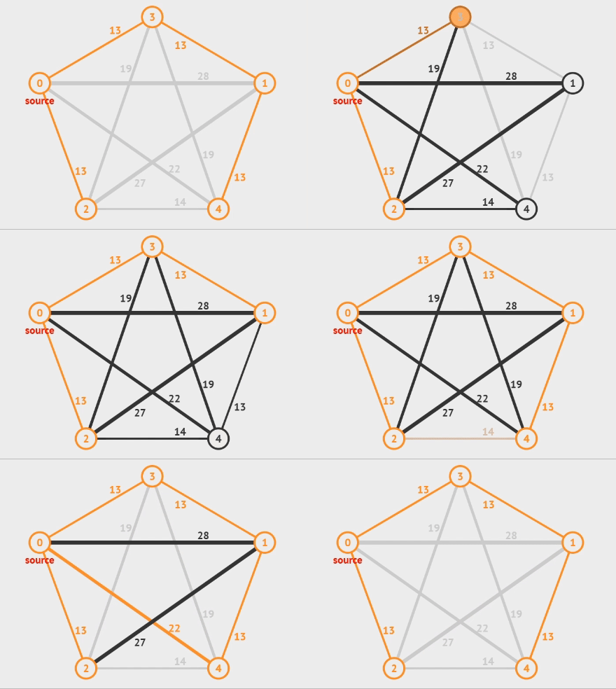
Prim’s Algorithm is an greedy algorithm.

Start with a tree $T$ composed of $1$ vertex
Grow the tree $T$ $T$ by repeatedly adding the least weight edge $(u, v)$ $(u, v)$ until it has $n-1$ $n - 1$ edges
- Only one of $u$ and $v$ is in $T$

Pseudo Code

// From VisuAlgo
T = {s}

enqueue edges connected to s in PQ (by inc weight)

while (!PQ.isEmpty)

    if (vertex v linked with e = PQ.remove ∉ T)

        T = T ∪ {v, e}, enqueue edges connected to v

    else ignore e

MST = T

Hash Tables

Intro

A table to store dictionary pairs
- A dictionary pair includes (key, value)
- Different pair has different key
Operations
- Search(key)
- Insert(key, value)
- Delete(key)
Expected Time
- $O(1)$

Example

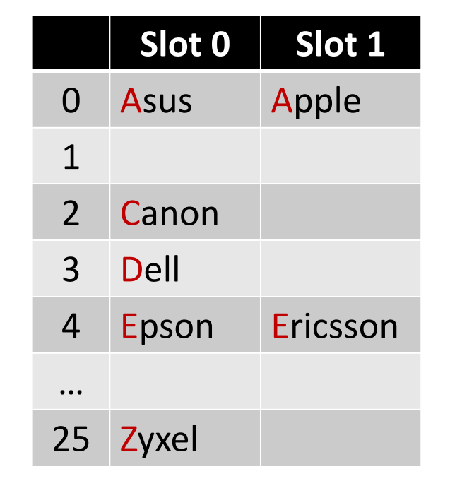
Insert the pairs with the following keys to the hash table. Asus, Canon, Zyxel, Epson, Ericsson, Apple, Dell

Hash Table ht
- 26 buckets (26 alphabets)
- 2 slots per bucket (like “a” bucket holds 2 pairs, Asus & Apple)
Hash Function h(k)
- Map the first character of a key from $0$ to $25$

Loading Density

Loading Density
- $\alpha=n/sb$
- $n$ is number of pairs in the table
- $s$ is number of slots per bucket
- $b$ is number of buckets

So in the previous example, we have the loading density $\alpha=7/(2\times26)$ .

Synonyms

$2$ $2$ keys are synonyms if h(k1)==h(k2)
- In the previous example, Asus and Apple are synonyms
When Inserting Pairs in Previous Example
- Insert(Cisco, 1000)
  - The home bucket isn’t empty
  - Collision
- Insert(Acer, 1000)
  - The home bucket is full
  - Overflow
- Collision & Overflow occur simultaneously when each bucket has only $1$ slot

Ideal Hash Functions

Easy to compute
Minimize number of collisions
No biased use of hash table
- h(k) is independently and uniformly at random from $0$ to $b-1$
- The probability of a bucket to be selected is $1/b$

Hash Functions: Division

Division
- $h(k)=k\pmod D$
- Use the remainder
- Have at least $D$ buckets in the hash table
Example
- Inserting pairs $(22,a), (34,c), (3,d), (73,e), (86,f)$
- Hash table with $11$ slots, ht[0:10]
- Hash function: $key\pmod{11}$

Hash Functions: Folding

Partition the key into several parts $P_0, P_1, \dots, P_i$ and add all partitions together
Shift folding
- $h(k)=P_0+P_1+\dots+P_i$
- $k = 12320324111220$ and we partition it into $3$ digits long, then $h(k)= 123 + 203 +241 +112 +20 = 699$
Folding at the boundaries
- Reversing every other partition and then adding
- $k=12320324111220$ and we partition it into $3$ digits long, then $h(k) = 123 + 302 +241 +211 +20 = 897$

Overflow Handling

Chaining

Intro

A linked list per bucket
Each list contains all synonyms
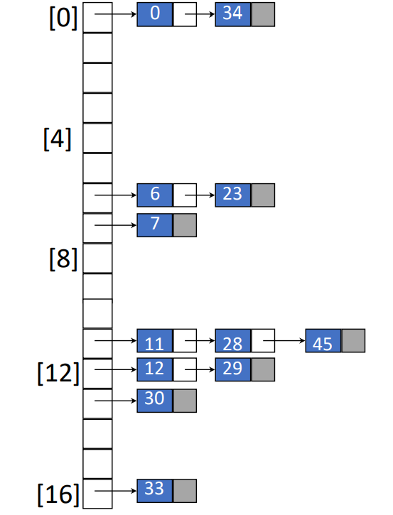
Example
- Inserting pairs whose keys are $6, 12, 34, 29, 28, 11, 23, 7, 0, 33, 30, 45$
- Hash function is $h(key)=key\pmod{17}$
Average chain length is $n/b$

Expected Performance

If we have a chained hash table with uniform hash functions

Average chain length is $\frac{n}{b}$ $\frac{n}{b}$
- $n$ is number of data items in hash table
- $b$ is the number of buckets (number of chains)
$U_n$ $U_{n}$
- Expected number of key comparisons in an unsuccessful search
- Expected nubmer of keys on a chain
- $U_n=\frac{n}{b}$
$S_n$ $S_{n}$
- Expected number of key comparisons in a successful search
- When the $i^{th}$ key is being inserted, the expected number of keys in a chain is $\frac{(i-1)}{b}$
- The expected number of comparisons needed to search for $k_i$ is $1+\frac{i-1}{b}$ . (Assuming that new entry will be insert)
- Find the $i^{th}$ $i^{t h}$ key, averaged over $1\le i\le n$ $1 \leq i \leq n$
  - $S_n=\frac{1}{n}\displaystyle\sum^n_{i=1}\{1+\frac{i-1}{b}\}\approx 1+\frac{\alpha}{2}$

Open Addressing

Search the hash table in some systematic fashion for a bucket that is not full
- Linear probing (linear open addressing)
- Quadratic probing
- Rehashing
- Random probing

Linear Probing

Search

Search the hash table in the following order
- $ht[h(k)\bmod{b}],ht[(h(k)+1)\bmod{b}],\dots,ht[(h(k)+b)\bmod{b}]$
- $ht$ is hash table
- $h(k)$ is the hash function
- $b$ is the number of bucket

Insert

The insert terminate when we reach the first unfilled bucket
- Insert the pair into taht bucket

For example, we have a hash function $key\pmod{17}$ and $b=17$ . Insert pairs whose keys are $6, 12, 34, 29, 28, 11, 23, 7, 0, 33, 30, 45$

Index	0	1	2	3	4	5	6	7	8	9	10	11	12	13	14	15	16
Value	34	0	45				6	23	7			28	12	29	11	30	33

Delete

In linear probing, we cannot directly delete an element in the hash table. Since if we do that, the corresponding position will be None, that way, the search function will return when encounter the None, so all the elements after None won’t be visited. To solve it, we use Tombstone to replace the none, we put a Tombstone in the element place we want to delete, and this is call lazy deletion.

Expected Performance

Loading density of a hash table takes $\alpha = n/b$
- $n$ is number of data item in hash table
- $b$ is number of buckets
When $n$ is large and $0\le\alpha\le 1$
- $U_n$ $U_{n}$
  - Expected number of key comparisons in an unsuccessful search
  - $U_n\approx\frac{1}{2}\{1+\frac{1}{(1-\alpha)^2}\}$
- $S_n$ $S_{n}$
  - Expected number of key comparisons in a successful search
  - $S_n\approx\frac{1}{2}\{1+\frac{1}{1-\alpha}\}$
$\alpha\le0.75$ is recommended
- Proven by Knuth, 1962
- $\alpha$ $S_n$ $U_n$
  $0.50$ $1.5$ $2.5$
  $0.75$ $2.5$ $8.5$
  $0.90$ $5.5$ $50.7$

$\alpha$	$S_n$	$U_n$
$0.50$	$1.5$	$2.5$
$0.75$	$2.5$	$8.5$
$0.90$	$5.5$	$50.7$

Quadratic probing

In quadratic probing, we search elements in the following order. ( $h$ is hash function, $b$ is number of buckets)

$\begin{aligned} &ht[h(k) \bmod b],\\ &ht[(h(k)+1) \bmod b], ht[(h(k)-1) \bmod b],\\ &ht[(h(k)+2^2) \bmod b], ht[(h(k)-2^2) \bmod b],\\ &ht[(h(k)+3^2) \bmod b], ht[(h(k)-3^2) \bmod b], \\ &\vdots \\ \end{aligned}$

For example, if $h(k)=k\bmod b$ , where $b=7$

$k = 2$ $k = 2$
- $h(k) = 2, \quad\text{Probing sequence is}\quad \{2, 3, 1, 6, 5, 4, 0\}$
$k = 6$ $k = 6$
- $h(k) = 6, \quad\text{Probing sequence is} \quad\{6, 0, 5, 3, 2, 1, 4\}$
$k = 19$ $k = 19$
- $h(k) = 5, \quad\text{Probing sequence is}\quad \{5, 6, 4, 2, 1, 0, 3\}$

Rehashing

Create a series of hash functions $h_1, h_2, h_3, \dots, h_m$
Examine buckets in the order of $h_1(k), h_2(k), h_3(k), \dots, h_m(k)$

Perfomances

Worst case for find/insert/delete time is $O(n)$ $O (n)$ , $n$ $n$ is the number of pairs in the table
- Open addressing
  - This happens when all pairs are in the same cluster
- Chaining
  - This happens when all pairs are in the same chain

Bloom Filters

Intro

When
- Returning maybe and No are acceptable
What
- Bit array
- Uniform and independent hash functions $f_1, f_2, \dots, f_h$
Limitations
- The naive implementation of the bloom filter doesn’t support the delete operation
- The false positives rate can be reduced but can’t be reduced to zero

Operations

Insert(k)

Given $m$ bits of memory $BF$ and $h$ hash functions, then $0\le f_i(k)\le m-1$

Initialize all $m$ bits to be $0$
To insert key $k$ , set bits $f_1(k), f_2(k), f_3(k),\dots,f_h(k)=1$
So $1$ key will make multiple indices changes

Member(k, BF)

Search for key $k$

ANY $BF[f_i(k)]=0$ means $k$ is not in the set
ALL $BF[f_i(k)]=1$ means $k$ may be in the set

Performances

Assume that a bloom filter with

$m$ bits of memory
$h$ uniform hashed functions
$u$ elements

Consider the $i^{th}$ bit of the bloom filter

Probability to be selected by the $j^{th}$ $j^{t h}$ hash function $f_j(k)$ $f_{j} (k)$
- $P[f_j(k)=i]=\frac{1}{m}$
Probability of unselected by the $j^{th}$ $j^{t h}$ hash function $f_j(k)$ $f_{j} (k)$
- $P[f_j(k)\ne i]=1-\frac{1}{m}$
Probability of unselected by any of $h$ $h$ hash functions
- $1\le j\le h, P[f_j(k)\ne i]=(1-\frac{1}{m})^h$
After inserting $u$ $u$ elements, probability of unselected by any of $h$ $h$ hash functions
- $p = (1-\frac{1}{m})^{h\cdot u}$
After inserting $u$ $u$ elements, probability that bit $i$ $i$ remains $0$ $0$
- $p=(1-\frac{1}{m})^{h\cdot u}$
After inserting $u$ $u$ elements, probability that bit $i$ $i$ is $1$ $1$
- $1-p$

Probability of false positives

Take a random element $k$ and check $Member(k, BF)$
The probability that all $h$ $h$ bits $f_1(k),\dots, f_h(k)$ $f_{1} (k), \dots, f_{h} (k)$ in $BF$ $BF$ are $1$ $1$
- $f = (1-p)^h$

Design of Bloom Filters

Choose $m$ $m$ (filter size in bits)
- Large $m$ to reduce filter error
Pick $h$ $h$ (number of hash functions)
- $h$ $h$ is too small
  - Probability of different keys having same signature is high
  - Test more bits for $Member(k, BF)$ $M e mb er (k, BF)$
    - Lower false positive rate
  - More bits in $BF$ $BF$ are $1$ $1$
    - Higher false positive rate
- $h$ $h$ is too large
  - The bloom filter fills with ones quickly
  - Test less bits for $Member(k, BF)$ $M e mb er (k, BF)$
    - Higher false positive rate
  - More bits in $BF$ $BF$ are $0$ $0$
    - Lower false positive rate
Select $h$ $h$ hash functions
- Hash functions should be relatively independent

Given $m$ bits of memory and $u$ elements, choose $h=\frac{m\ln 2}{u}$

Probability that some bit $i$ $i$ is $1$ $1$
- $p\approx e^{\frac{-h \cdot u}{m}}=\frac{1}{2}$
Expected distribution
- $\frac{1}{2}$ bits are $1$ and vice versa
Probability of false positives
- $f=(1-p)^h\approx(\frac{1}{2})^h=(\frac{1}{2})^{(\ln 2)\frac{m}{u}}\approx 0.6185^{\frac{m}{u}}$

Minimize The False Positive Rate

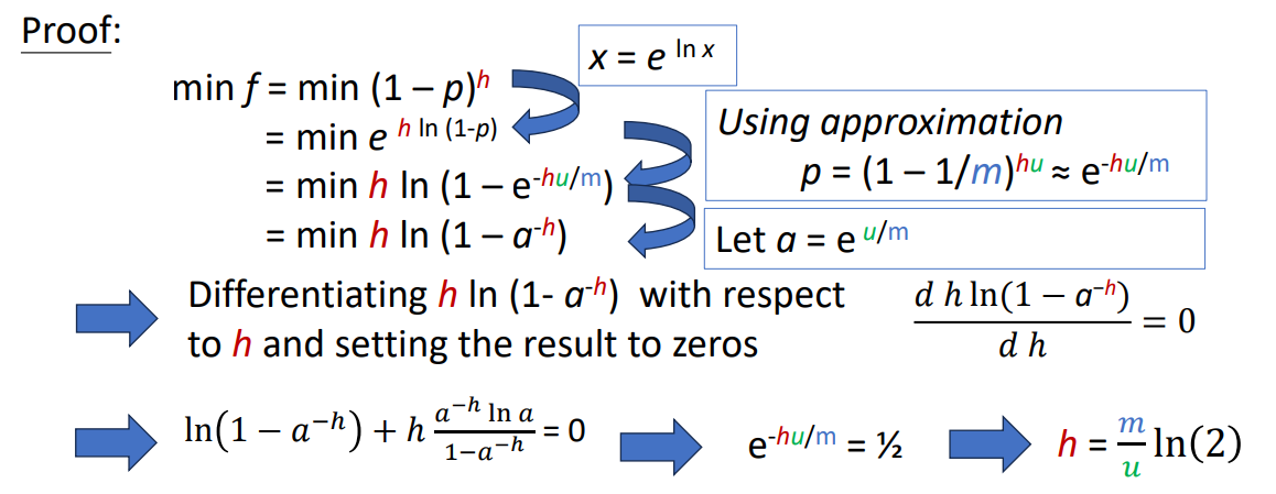
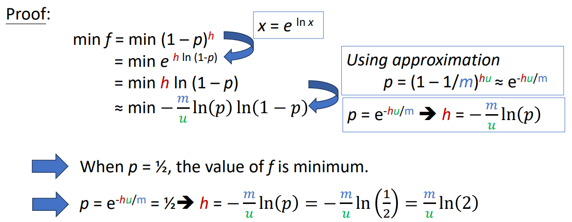
Assume that the filter size $m$ and the number of elements in the filter $u$ are fixed, $h$ minimizes false positive rate $f$ if

$h = \frac{(m \ln 2)}{u}$

Proof 1

Proof 2

Binomial Heaps

Leftist vs Binomial Heaps

This is a table of time complexity for different operations.

Operations	Leftist Heaps	Actual Binomial Heaps	Amortized Binomial Heaps
Insert	$O(\log n)$	$O(1)$	$O(1)$
Delete min (or max)	$O(\log n)$	$O(n)$	$O(\log n)$
Meld	$O(\log n)$	$O(1)$	$O(1)$